How to turn outpainted image sequences created by Midjourney or other generative AI's into videos with an infinite zoom effect.
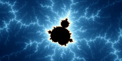
An introduction to Benoît Mandelbrot's Wonderful World of Fractals.


Evolution, is the change in heritable phenotype traits of biological populations over successive generations. Evolutionary processes give rise to diversity at every level of biological organization, including the level of species, individual organisms, and at the level of molecular evolution.
This article deals with the simulation of artificial life by using basic principles of evolution. The simulation presented here is a modified versions of a program first described by Michael Palmiter [1]. and later popularized by A. K. Dewdney in an article series published in the Scientific American magazine [2]. The simulation demonstrates the evolution of hunting behavior in an predator/prey situation. The simulation domain represents a small patch of a lake bottom. Microbes move across the screen living off a supply of bacteria. The bacteria are the only source of energy. The motion of a microbe is determined by a set of genes. The genes control the probability with wich a microbe will change its direction at a given time step.
To create an evolution simulator we need a species with an easily observable behavioral pattern that is determined by a small set of genes. In the simulation laid out here the genes determine the preferred motion of a microbe. An individual competes with other members of the species for a food supply. If enough food was consumed by an individual it may create offspring after a certain amount of time. The offspring will have a slightly modified set of genes based on the parent genes. This implies that organisms which are successful in their search for food have a higher chance of creating offspring an thus passing on their genes.
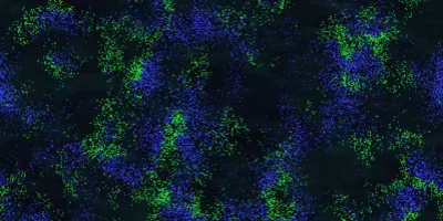
The simulation deals with microbes living off an unlimited but randomly distributed food supply. The microbes live on a two dimensional grid. They can move freely into any of the eight neighboring cells. The edges of the grid are connected. If a microbe moves across the edge of the grid it immediately enters the grid back again on the opposing side. Microbes are rendered in blue, whilst food is rendered in green. For the sake of clarity microbes are rendered larger than the food but in terms of the simulation they still only occupy a single cell. There is no limit as to how many microbes a grid cell can contain. If multiple microbes are present they will be rendered above each other appearing as a single one.
 Image 1: Microbes living on a grid that contains randomly distributed food sources.
The simulation runs in discrete time steps. In each time steps the microbes move along a straight line following their current direction of motion. If a microbe enters a cell occupied by food the food is consumed and the microbe gains a bit of additional energy. If multiple microbes enter the same cell in the same time step the first one to enter gets to eat the food.
Microbes constitute the active part of the simulation they move along the grid and they are subject to evolution during the course of the simulation.
Microbes can move freely to their neighboring cells. They travel alongside one of eight possible directions of motion. The motion direction is stored as an integer value. This value is used as an index to look up the specific ΔX and ΔY step sizes for moving over the grid. Motion is then implemented by adding these delta values to the current microbe grid position. The motion table is set up in a way that only motions to neighboring cells are possible.
 Image 2 Left: The eight possibilities of moving a microbe; Right: Motion table with the corresponding motion step data.
| Direction Index | Grid Steps | |
|---|---|---|
| Δx | Δy | |
| 0 | -1 | 1 |
| 1 | 0 | 1 |
| 2 | 1 | 1 |
| 3 | -1 | 0 |
| 4 | 1 | 0 |
| 5 | -1 | -1 |
| 6 | 0 | -1 |
| 7 | 1 | -1 |
At every time step there is a certain probability with which a microbe will change its direction into another direction. The probabilities of all possible transitions represent the genome of the microbe. The genes will be labeled with the letter p and an index. The sum of all probabilities (genes) is one: \[\sum_{n=0}^7 p_n = 1\]
Each gene represents a segment of the interval [0,1] whose length is proportional to the gene value. The following example shows a random genome in which the gene sizes are rendered proportional to their value. Each gene represents the likelihood of a certain change in direction:
In order to compute the new direction with a probability proportional to the corresponding gene value a random value r between 0 and 1 is computed:
\[r = rnd(1)\]Then the index i of the gene is computed. This index is the smallest possible i for which the following inequality holds true:
\[r \lt \sum_{n=0}^i p_{n}\] I the example above i equals 3. This is the index of the directional change be applied. The direction d of the microbe in the next time step is then computed by adding i to the current direction and determining the remainder of the division by 8 (the total number of possible changes): \[d_{t+1} = (d_{t} + i)\mod 8\]With this equation we can easily deduce the meaning of each of the genes:
| Gene | Function | |
|---|---|---|
| Index i | Identifier | |
| 0 | p0 | No change |
| 1 | p1 | light turn to the right |
| 2 | p2 | right turn |
| 3 | p3 | hard right turn |
| 4 | p4 | reverse |
| 5 | p5 | hard left turn |
| 6 | p6 | left turn |
| 7 | p7 | light left turn |
 Image 3: Two images illustrating the amount of energy needed to change the direction of two microbes traveling in different directions.
The required energy depends on the extend of the turn. Continuing the motion without change is free.
Image 3: Two images illustrating the amount of energy needed to change the direction of two microbes traveling in different directions.
The required energy depends on the extend of the turn. Continuing the motion without change is free.
Each microbe has a finite amount of energy and with each time step a small fixed amount of energy is subtracted to account for the "energy cost" of living and moving. In addition changing the direction also requires energy. The more drastic the directional change is the more energy is required. A microbe can boost its energy by consuming food. It needs a constant supply of food in order to continue living since it will die if it has exhausted its energy supply. A microbe stops eating once it has gained a certain amount of energy.
Once a microbe has reached a certain age it will create offspring if it has enough energy. The energy is evenly split between the parent and the child. The child will start with a genome that is based on the parents genome but contains a single slightly modified gene. The following table provides an overview on the parameters related to the microbes energy management:
| Parameter | Value |
|---|---|
| Energy gain per food item | 40 |
| Maximum Energy | 1500 |
| Maximum needed to Reproduce | 1000 |
| Energy lost per time tick | 1 |
| Energy required for changing the direction | see Image 3 |
The food supply is unlimited. Each grid cell can either be empty or contain food. Food does not have a life cycle of its own. If a cell contains food it remains there until a microbe eats it. In order to put the population under evolutionary stress The simulation can spawn the food in three distinct patterns:
 Option 1: Randomized food distribution.
 Option 2: Food spawns primary along vertical and horizontal.
 Option 3: Food spawns primary in a rectangle in the center of the simulation domain.
The simulation starts with plenty of food and few microbes. At first the genes are set randomly. The microbes do not have a prefered direction. They are aimlessly wandering around effectively remaining on the same spot due to running in small circles. In the beginning this is fine because there is plenty of food. No matter how clumsy a microbe is moving it will find enough food to reach the energy level needed to start procreating. More microbes are created and suddenly the parent is competing with the child for food. Both are at the same spot and both are hardly moving into any direction. The local food supply is rapidly dwindling and it is now advantageous to be able to move away from the competition. Microbes which are equipped with genes that allow for fewer direction changes suddenly have an competitive advantage. They spend fewer energy for changing their direction an they can reach yet untouched areas of the simulation domain.
Soon an equilibrium is reached and the population is more or less stable. Microbes travel longer distances in straight lines with an occasional change in direction. The simulation is now a typical predator-prey interaction similar to the Wator simulation.
 Image 5: With evenly distributed food supply microbes quickly learn to move in straight line for small periods of time. This allows them to reach
regions with more food and escape local competition.
Image 5: With evenly distributed food supply microbes quickly learn to move in straight line for small periods of time. This allows them to reach
regions with more food and escape local competition.
The next scenario is often called the "Garden of Eden" scenario. Food is spawning randomly across the map but there is a small rectangular region in the middle of the simulation domain with a drastically increased supply of food. Soon microbes reaching this region will exhibit a wildly spinning behavior to avoid leaving the food supply. A degeneration in the genom causes microbes to constantly change their directions. On average they remain at their position by wildly going in circles. The reason is simple: Only microbes unable of leaving the Garden of Eden will benefit from its unlimited food supply in the long term.
Outside the "Garden of Eden" there is still food spawning but to a lesser degree. Some microbes will adapt to survive there. Food is sparse there and again the microbes living there are forced to wander long distances in order to survive. In a way its like seeing two different specied evolve due to natural selection.
 Image 6: The Garden of Eden. A degeneration in the genom causes microbes to constantly change their directions. On average they remain at their position by
wildly going in circles. Only microbes unable of leaving the garden of eden will benefit from its unlimited food supply in the long term.
Image 6: The Garden of Eden. A degeneration in the genom causes microbes to constantly change their directions. On average they remain at their position by
wildly going in circles. Only microbes unable of leaving the garden of eden will benefit from its unlimited food supply in the long term.
What happens if we push the "Garden of Eden" scenario to an extreme? Lets say by almost exclusively spawning food along a few horizontal and vertical lines. Some food will also spawn elsewhere but not much. At first the microbes resort to their most basic strategy: Reducing the number of direction changes and travel long distances in order to survive by increasing the chance of finding food elsewhere. This will go on for quite some time until one of the microbes accidentally finds a line full of food. It will wander along this line and receive a sudden boost of energy resulting in a drastically increased chance of procreation. The longer it travels along the line the greater the benefit. Soon it will leave the line again but it will also have created offspring that has a slightly higher probability to walk longer distances in a straight line than the rest of the population. This will continue for quite some time resulting in a gradual decrease in the ability to change the direction.
At some point in time one of the descendants will find a line again. The genome is now set up in a way that very few direction changes take place. The energy boost from finding the line will reduce the probability even more in some of its descendants. They will eventually loose the ability to move away from the line altogether. From this point on a new species of "Line Riders" will populate the line. Soon other lines will follow until the "Line Riders" become the dominant species in the simulation.
 Image 7: Spawning food primarily along horizontal and vertical lines will eventually lead to the creation of a species of "Line Riders" that live on the linear
food spawning areas.
Image 7: Spawning food primarily along horizontal and vertical lines will eventually lead to the creation of a species of "Line Riders" that live on the linear
food spawning areas.
The evolution simulator is part of the Educational-Javascripts-Typescript repository at GitHub. In order to run it a HTML 5 capable browser is needed. I recommend using a Javascript Debugger like Firebug (for Firefox Browser) in order to play with the code.
How to turn outpainted image sequences created by Midjourney or other generative AI's into videos with an infinite zoom effect.
An introduction to Benoît Mandelbrot's Wonderful World of Fractals.
Fully automated article generation on arbitrary topics using artificial intelligence with OpenAi's GPT-4 and Python.
Learn about predator-prey-interactions in the toroidal world of Wator.
Nuclear chain reactions in gun type atomic bombs - How did the Hiroshima Bomb work?