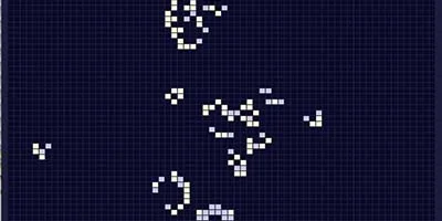
An implementation of John Conway's Game of Life in Python.

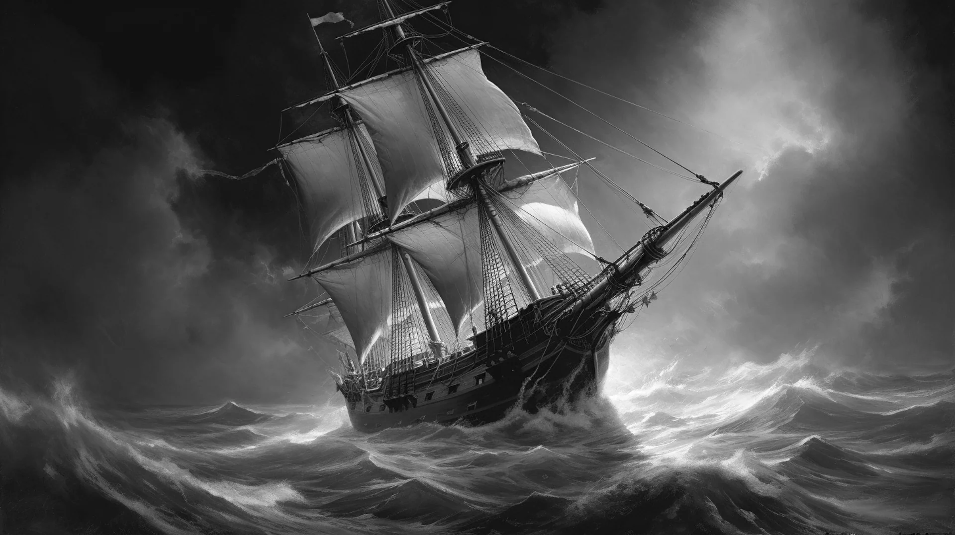
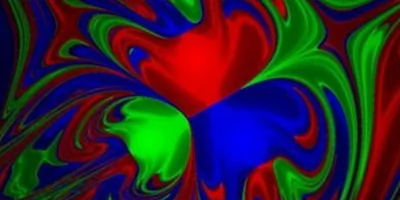
How simple dots create digital works of art
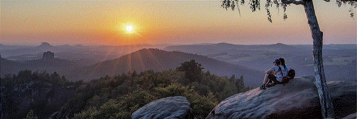 This image uses only 8 colors in total. Through dithering, the impression of a much higher color depth is created.
For display in the browser a slight blur was added in order to avoid the moiré effect.
It works much like on analog television sets, whose sharpness was likewise limited. In fact,
computer games used to look better on CRT monitors than on the high-resolution displays of today.
This image uses only 8 colors in total. Through dithering, the impression of a much higher color depth is created.
For display in the browser a slight blur was added in order to avoid the moiré effect.
It works much like on analog television sets, whose sharpness was likewise limited. In fact,
computer games used to look better on CRT monitors than on the high-resolution displays of today.
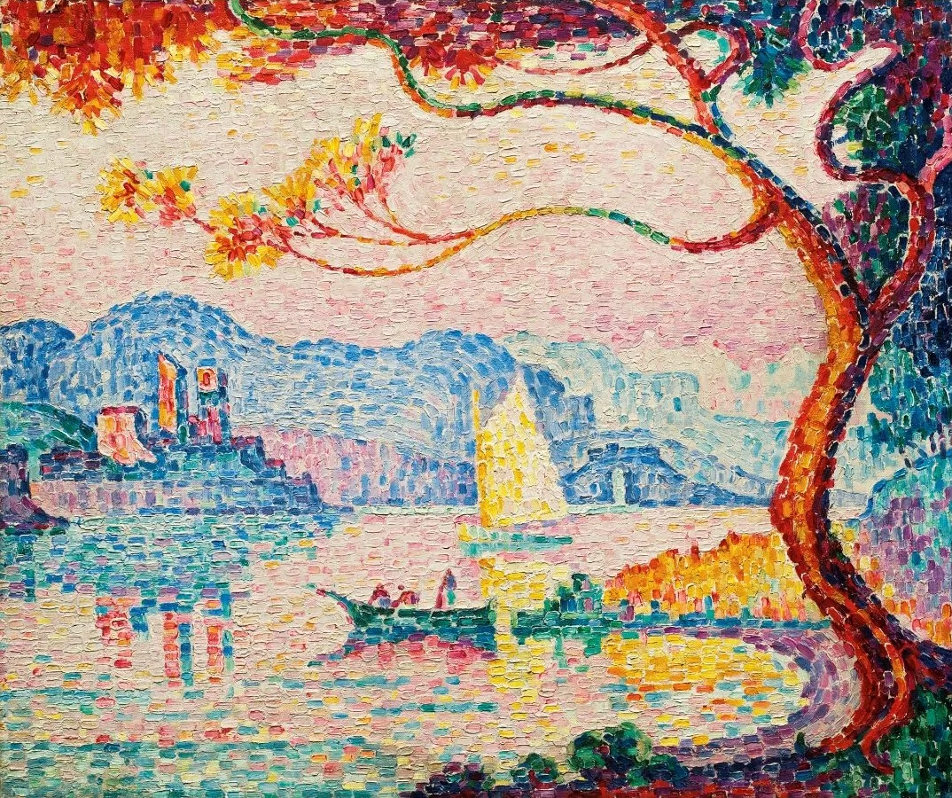 The Impressionists already played with creating colors through neighboring colored dots.
Shown here in the painting "Antibes. Petit Port de Bacon." — a pointillist painting by
Paul Signac from 1917. (via Wikimedia Commons; public domain)
The Impressionists already played with creating colors through neighboring colored dots.
Shown here in the painting "Antibes. Petit Port de Bacon." — a pointillist painting by
Paul Signac from 1917. (via Wikimedia Commons; public domain)
At the beginning of the 1980s, home computers began their triumphal march into the living rooms of the world. Their graphical capabilities, in terms of both screen resolution and color palette, were limited. This presented developers and graphic designers with the challenge of realizing their creative ideas on this constrained hardware. How do you depict an impressive sunset using only 2, 4 or 16 colors?
The answer is dithering, also known as error diffusion. It is an image-processing technique that, by cleverly placing colored pixels next to one another, creates the illusion of a greater color depth. Computer artists borrowed the trick from the French Impressionists, who had already discovered how the placement of small patches of color side by side can create the illusion of a different color. A drawing technique that was initially dismissed under the disparaging label "pointillism".
One hundred years later, in the 1980s, the technique was rediscovered or, rather, reinvented. The limited graphical capabilities of home computers gave it new use cases, and with computer games entering the mainstream, there was finally a market for it as well.
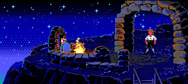 "The Secret of Monkey Island" (1990) by Lucasfilm Games. The on-screen graphics of the 16-color PC EGA
version show the typical patterns of ordered dithering in the sky.
"The Secret of Monkey Island" (1990) by Lucasfilm Games. The on-screen graphics of the 16-color PC EGA
version show the typical patterns of ordered dithering in the sky.
Today the circle has closed. Dithering has once again become an artistic design element. It is used to achieve the 8-bit retro look in modern video games or to create entirely new games with a unique aesthetic, such as "Return of the Obra Dinn". For better computer graphics it is no longer needed, since modern graphics cards have long since stopped having any noticeable display limitations.
The problem of color reduction shall be illustrated by way of an example. Consider a digitized image that may contain up to 16,777,216 possible colors. This number comes from the fact that color information in JPEG images is stored across the three color channels red, green and blue. Each color channel can take on 256 different brightness values. That gives a total of 256 × 256 × 256 = 16,777,216 different possible colors. We want to optimize the image for display on a monochrome monitor. This monitor can only display black and white pixels.
In a first step, we convert the image to grayscale. Using a threshold algorithm we then turn it into a black-and-white image. The algorithm compares the brightness of each pixel of the grayscale image to a threshold value and turns the pixel white if it is above the threshold or black if it is below.
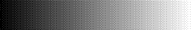
 We start with a grayscale image. This image has 8-bit color depth, which translates into 256 different
brightness levels per pixel.
We start with a grayscale image. This image has 8-bit color depth, which translates into 256 different
brightness levels per pixel.
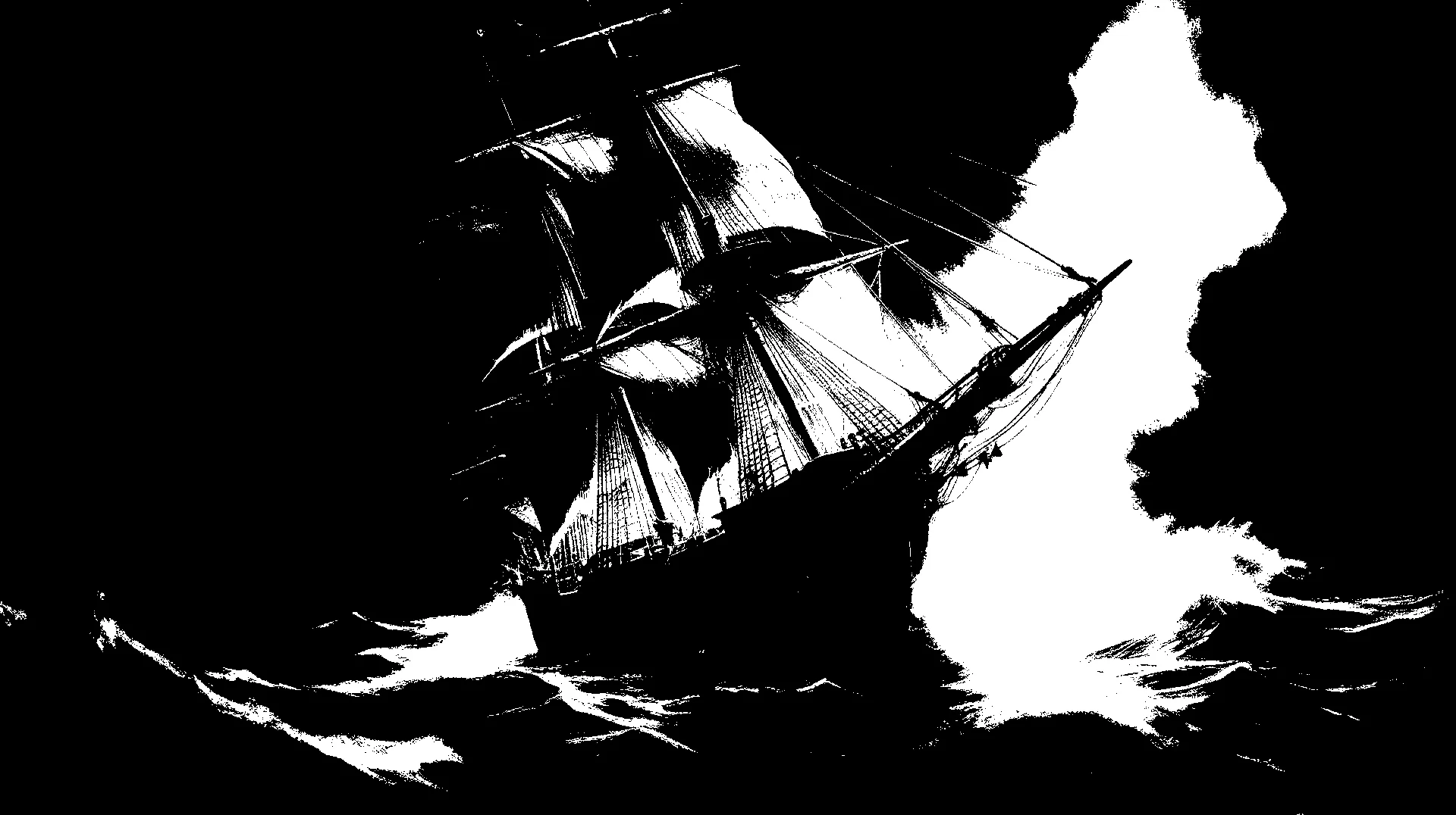 Threshold algorithms are not well suited for converting images into black-and-white images, because
local brightness information is almost completely lost.
Threshold algorithms are not well suited for converting images into black-and-white images, because
local brightness information is almost completely lost.
The result is disappointing. The image is barely recognizable. It shows large monochrome areas in which all detail is lost (so-called "banding"). One could try to vary the threshold, but this would not help much. Local image information is lost completely once the contrast becomes too low.
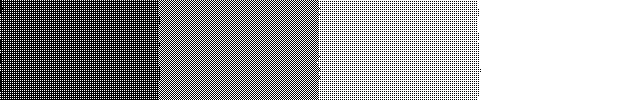 With a 2×2 Bayer matrix, 4 different patterns can be produced for a brightness gradient.
 With a 4×4 Bayer matrix, 16 different patterns are possible.
 With an 8×8 Bayer matrix, 64 different patterns are possible.
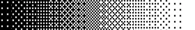
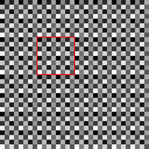 Threshold map based on an 8×8 Bayer matrix that has been tiled. The red square marks one cell.
Ordered dithering is an improvement over the simple threshold algorithm. It is based on a threshold comparison against a threshold map that is built from a predefined matrix. This matrix is called a Bayer matrix. Bayer matrices can be computed in different sizes. The larger the matrix, the more brightness gradations it can represent.
2×2 Bayer matrix \begin{equation} \mathbf{M}=\frac{1}{4}\begin{bmatrix}0 & 2 \\3 & 1\end{bmatrix} \end{equation} 4×4 Bayer matrix \begin{equation} \mathbf{M}=\frac{1}{16}\begin{bmatrix}0 & 8 & 2 & 10 \\ 12 & 4 & 14 & 6 \\ 3 & 11 & 1 & 9 \\ 15 & 7 & 13 & 5 \end{bmatrix} \end{equation} 8×8 Bayer matrix \begin{equation} \mathbf{M}=\frac{1}{64}\begin{bmatrix}0 & 32 & 8 & 40 & 2 & 34 & 10 & 42\\ 48 & 16 & 56 & 24 & 50 & 18 & 58 & 26 \\ 12 & 44 & 4 & 36 & 14 & 46 & 6 & 38 \\ 60 & 28 & 52 & 20 & 62 & 30 & 54 & 22 \\ 3 & 35 & 11 & 43 & 1 & 33 & 9 & 41 \\ 51 & 19 & 59 & 27 & 49 & 17 & 57 & 25 \\ 15 & 47 & 7 & 39 & 13 & 45 & 5 & 37 \\ 63 & 31 & 55 & 23 & 61 & 29 & 53 & 21 \end{bmatrix} \end{equation}For images with 8-bit color depth, the matrices still need to be multiplied by 256. The 2×2 Bayer matrix with thresholds for 8 bits therefore reads:
\begin{equation} \mathbf{M}=\begin{bmatrix}0 & 128 \\192 & 64\end{bmatrix} \end{equation}The threshold map is created by tiling the Bayer matrix in x and y until it has the same resolution as the image whose colors are to be reduced. For dithering, every pixel of the original image is then compared with the corresponding value in the threshold map. If it is greater, the pixel becomes white; if it is smaller, the pixel becomes black. [3]
Dithering with a 2×2 matrix is not convincing. Four patterns for the representation of grayscale values are too few; however, the subject is now at least recognizable. The image with an 8×8 matrix is better and looks fairly okay. Even so, this kind of dithering produces visually distracting, repeating patterns.
 Ordered dithering with a 2×2 Bayer matrix. The quality is not convincing. Banding is still visible,
but now with monochrome patterns.
Ordered dithering with a 2×2 Bayer matrix. The quality is not convincing. Banding is still visible,
but now with monochrome patterns.
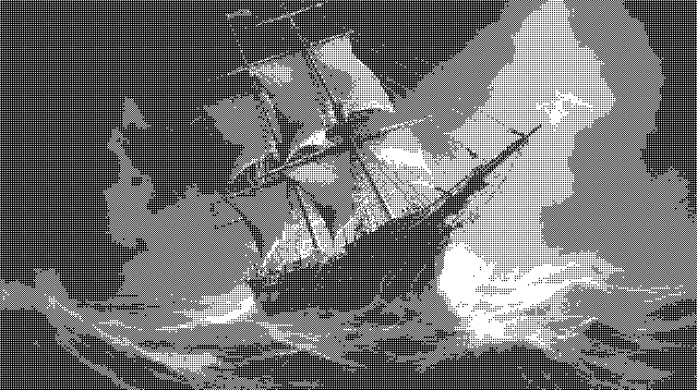
 Ordered dithering with an 8×8 Bayer matrix. The subject is rendered more clearly, but distracting,
regular patterns appear.
Ordered dithering with an 8×8 Bayer matrix. The subject is rendered more clearly, but distracting,
regular patterns appear.
Dithering with Bayer matrices is still occasionally used today, but better methods exist. Even though the results are not stunning, a decisive advantage of this method is its simplicity. Algorithmically, it is for example very well suited to implementation on the shaders of modern graphics cards.
With Bayer matrix dithering, gray values are converted into black and white pixels by a brightness comparison against a threshold map. The threshold maps were generated by tiling the Bayer matrices. This led to distracting, repetitive patterns in the resulting image.
What could be more obvious than to "randomize" the threshold map in order to break up these patterns? Not for nothing does the term "dithering" derive from the English word for "to tremble". For a simple implementation in Python, every pixel of the source image is compared against a randomly chosen brightness value. If the pixel's brightness is greater, it becomes white; if smaller, it becomes black.
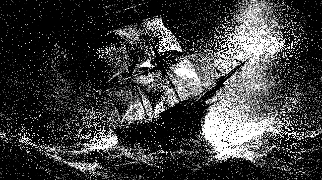 Dithering with normally distributed random numbers. For comparability the same resolution was used as
for the Bayer matrix examples.
Dithering with normally distributed random numbers. For comparability the same resolution was used as
for the Bayer matrix examples.
def dither_noise(gray_img):
    height, width = gray_img.shape

    for y in range(height):
        for x in range(width):
            old_pixel = gray_img[y, x]
            new_pixel = 0 if old_pixel < random.randint(0, 255) else 255
#            new_pixel = 0 if old_pixel < int(np.random.normal(127, 64)) else 255
            gray_img[y, x] = new_pixel

    return gray_img
It makes sense to keep 127 as the threshold, since this is the midpoint of the brightness scale. One can experiment with different distributions of random numbers, but the result will not change qualitatively in any dramatic way. The ship is recognizable, but the result is rather noisy. Interesting effects can definitely be achieved with this kind of dithering when the resolution of the source image is large enough. Practical relevance, however, is limited.
To improve the result, we now turn to algorithms that take the quantization error into account and distribute it over neighboring pixels. Let us first look at a simple brightness gradient that is to be reduced to only two colors via a threshold algorithm.
 A brightness gradient from dark to bright over 10 pixels.
After applying the threshold filter, the first 7 pixels become black, because their values are smaller than 127, while the remaining three pixels become white. The sum of the quantization error across all 10 pixels is -200. That value is missing from the overall brightness of the pixel sequence. To get a better result one needs an algorithm that takes the quantization error into account and compensates for it.
 Application of a threshold filter with threshold value 127.
The first pixel has brightness 12 but is set to 0. The quantization error of this pixel is therefore -12.
The sum of the quantization error across all pixels is 200.
Application of a threshold filter with threshold value 127.
The first pixel has brightness 12 but is set to 0. The quantization error of this pixel is therefore -12.
The sum of the quantization error across all pixels is 200.
A simple error diffusion algorithm is to pass the quantization error on to the closest pixel. When processing from left to right, the error is added to the right-hand neighbor. This new value is then compared against the threshold and processed.
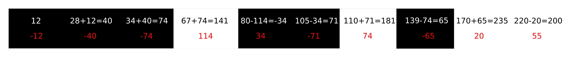 Transferring the quantization error onto the right-hand neighbor pixel.
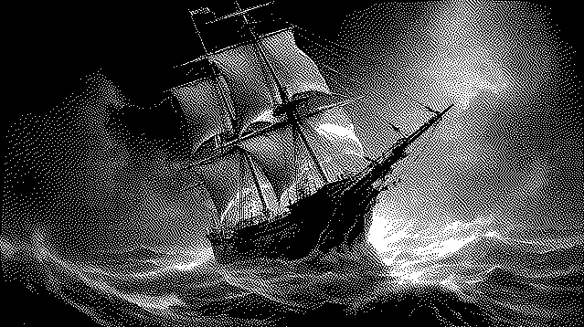
Applying this simple error diffusion algorithm to the example image produces the result shown below. Let's just say that it is not completely terrible. The ship is recognizable, but there are clear artifacts. Error diffusion takes place only along the X axis, and where similar gradients appear in the rows, the correction pixels also end up at similar positions. As a result, distinct vertical line structures appear.
 A simple dithering algorithm with error diffusion exclusively along the X axis.
An obvious improvement is to distribute the quantization error in 2 dimensions instead of just one.
 The Floyd-Steinberg algorithm distributes the quantization error onto neighboring pixels with different weights.
Dark gray pixels are the parts of the image that have already been processed. The dark blue cell is the current
cell, and the pale blue cells are the neighboring cells onto which the quantization error is distributed.
The Floyd-Steinberg algorithm distributes the quantization error onto neighboring pixels with different weights.
Dark gray pixels are the parts of the image that have already been processed. The dark blue cell is the current
cell, and the pale blue cells are the neighboring cells onto which the quantization error is distributed.
The most well-known error diffusion algorithm is the Floyd-Steinberg algorithm, published by Robert Floyd and Louis Steinberg in 1976. It and all the other algorithms described here process an image by iterating across all rows and columns. Every pixel is visited only once. Error diffusion is always applied in the forward direction of the rows and columns. Quantization errors can only be transferred to cells that have not yet been visited.
The algorithm uses only the four direct, not-yet-visited neighboring cells for error diffusion. As a result, it is relatively fast and can process the entire image in a single pass without the need for a buffer. Already processed pixels are not modified, while the pixels still to be processed are adjusted in accordance with the quantization errors that occur.
The following source code shows an implementation of the Floyd-Steinberg algorithm in Python.
def __dither_core_floyd_steinberg(gray_img):
	height, width = gray_img.shape

	for y in range(height):
		for x in range(width):
			old_pixel = gray_img[y, x]
			new_pixel = 255 if old_pixel > 127 else 0
			gray_img[y, x] = new_pixel
			error = old_pixel - new_pixel

			# Distribute the quantization error to the neighboring pixels, with rounding
			if x + 1 < width:
				gray_img[y, x + 1] = min(255, max(0, gray_img[y, x + 1] + int(error * 7 / 16)))
			if x - 1 >= 0 and y + 1 < height:
				gray_img[y + 1, x - 1] = min(255, max(0, gray_img[y + 1, x - 1] + int(error * 3 / 16)))
			if y + 1 < height:
				gray_img[y + 1, x] = min(255, max(0, gray_img[y + 1, x] + int(error * 5 / 16)))
			if x + 1 < width and y + 1 < height:
				gray_img[y + 1, x + 1] = min(255, max(0, gray_img[y + 1, x + 1] + int(error * 1 / 16)))

	return gray_img
The Floyd-Steinberg algorithm produces short, streak-like artifacts that, however, are rarely distracting and give it a characteristic look. For higher quality color reduction, additional algorithms were soon developed that distribute the quantization error over more than just the immediate neighbors.
In the years following 1980, a number of additional algorithms were proposed by various authors in quick succession. For home computers they came too late or were too computationally expensive. Floyd-Steinberg dithering and even Bayer matrices were good enough. On the other hand, the 1990s saw home computers replaced by PCs, whose VGA graphics cards could now display 256 colors out of 262,144 simultaneously. With more colors, the quality differences between the various dithering methods became less important. For a while, dithering still saw use in the creation of graphics for websites, since color reduction also reduced the file size of images.
 Atkinson algorithm
 Stucki algorithm
 Sierra algorithm
Algorithms worth mentioning include the Atkinson algorithm, developed by Bill Atkinson, a software engineer at Apple, which found broad use in that ecosystem. The algorithms by Peter Stucki and the Sierra algorithm by Frankie Sierra are likely among the highest-quality dithering algorithms.
 Floyd-Steinberg algorithm
 Atkinson algorithm
 Sierra algorithm
 Stucki algorithm
These algorithms can be implemented so that the dithering function takes a generic error distribution kernel as a matrix. For Floyd-Steinberg dithering the call to such a function would look like this:
kernel = np.array( [[0,  0,    0,   7/16, 0],
					[0, 3/16, 5/16, 1/16, 0],
					[0,  0,    0,    0,   0]] )
output = DitherProcessor.__dither_diffusion_generic_core(image, kernel)
The dithering function takes the kernel and distributes the error values to the neighboring pixels according to the kernel weights.
def __dither_diffusion_generic_core(gray_img, kernel):
	height, width = gray_img.shape

	for y in range(height):
		for x in range(width):
			old_pixel = gray_img[y, x]
			new_pixel = 255 if old_pixel > 127 else 0
			gray_img[y, x] = new_pixel
			quant_error = old_pixel - new_pixel

			# Distribute the quantization error to the neighboring pixels
			if x + 1 < width:
				gray_img[y, x + 1]     = min(255, max(0, gray_img[y, x + 1] + int(quant_error * kernel[0, 3])))
			if x + 2 < width:
				gray_img[y, x + 2]     = min(255, max(0, gray_img[y, x + 2] + int(quant_error * kernel[0, 4])))

			if y + 1 < height and x - 2 >= 0:
				gray_img[y + 1, x - 2] = min(255, max(0, gray_img[y + 1, x - 2] + int(quant_error * kernel[1, 0])))
			if y + 1 < height and x - 1 >= 0:
				gray_img[y + 1, x - 1] = min(255, max(0, gray_img[y + 1, x - 1] + int(quant_error * kernel[1, 1])))
			if y + 1 < height:
				gray_img[y + 1, x]     = min(255, max(0, gray_img[y + 1, x    ] + int(quant_error * kernel[1, 2])))
			if y + 1 < height and x + 1 < width:
				gray_img[y + 1, x + 1] = min(255, max(0, gray_img[y + 1, x + 1] + int(quant_error * kernel[1, 3])))
			if y + 1 < height and x + 2 < width:
				gray_img[y + 1, x + 2] = min(255, max(0, gray_img[y + 1, x + 2] + int(quant_error * kernel[1, 4])))

			if y + 2 < height and x - 2 >= 0:
				gray_img[y + 2, x - 2] = min(255, max(0, gray_img[y + 2, x - 2] + int(quant_error * kernel[2, 0])))
			if y + 2 < height and x - 1 >= 0:
				gray_img[y + 2, x - 1] = min(255, max(0, gray_img[y + 2, x - 1] + int(quant_error * kernel[2, 1])))
			if y + 2 < height:
				gray_img[y + 2, x]     = min(255, max(0, gray_img[y + 2, x    ] + int(quant_error * kernel[2, 2])))
			if y + 2 < height and x + 1 < width:
				gray_img[y + 2, x + 1] = min(255, max(0, gray_img[y + 2, x + 1] + int(quant_error * kernel[2, 3])))
			if y + 2 < height and x + 2 < width:
				gray_img[y + 2, x + 2] = min(255, max(0, gray_img[y + 2, x + 2] + int(quant_error * kernel[2, 4])))

	return np.clip(gray_img, 0, 255).astype(np.uint8)
Dithering of computer graphics is no longer necessary today. The arrival of display technologies such as e-paper, however, could give this technique something of a renaissance. E-paper displays are high-resolution passive displays whose pixels do not emit light themselves and are not lit from the front. The pixels can only represent a few brightness values. A perfect application for dithering!
 Monochrome video of a waterfall, created using dithering.
This article is based on information drawn from the following sources:
An implementation of John Conway's Game of Life in Python.
Learn how to write Stellarium scripts with Typescript.
Simulate the chaotic motion of a pendulum under the influence of gravity and three magnets.
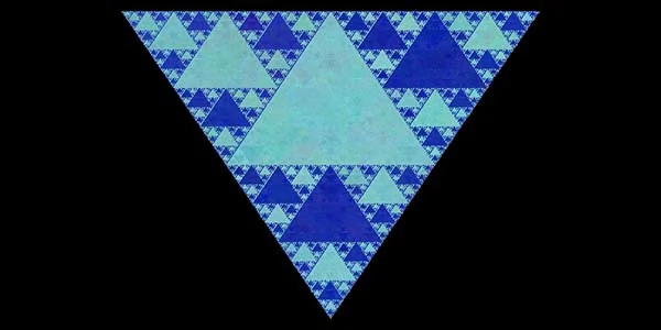
Learn how to create a colored version of the Siepinski-Triangle and many other fractals with recursive function calls.