Simulation of a predator/prey model on the toroidal planet Wator.


Evolution is the change in heritable traits of biological populations across many generations. Its core principle is natural selection: individuals carrying advantageous traits have a higher chance of producing offspring. This is often summarised as the "survival of the fittest".
This article deals with the simulation of very simple artificial life by applying basic evolutionary principles. The simulation shown here is a modified version of a program originally described by Michael Palmiter [1] and later popularised by A. K. Dewdney in a series of articles in Scientific American [2].
The scenario is the evolution of hunting behaviour in a predator/prey setup. Picture a small patch of sea floor: microorganisms drift across the simulation domain feeding on bacteria. The bacteria are their only source of energy. The motion of each microbe is determined by a set of genes that control the probability with which the microbe changes its direction in any given time step.
World: Color: Ticks/Frame Pause: Selection: Energy per food Max energy Reproduction threshold Energy per tick Food growth Visualisation of the genome of one microbe or of a group of microbes. The values of the
eight motion genes are shown as radial bars along their respective direction. In the centre
there is a magnified, coloured representation of a microbe whose colour is derived from the
same genome data.
Visualisation of the genome of one microbe or of a group of microbes. The values of the
eight motion genes are shown as radial bars along their respective direction. In the centre
there is a magnified, coloured representation of a microbe whose colour is derived from the
same genome data.
The genome of a microbe consists of 8 genes that govern the probability of changing direction into one of the eight possible directions of motion. In the upper right corner of the canvas these genes are visualised. When no microbe is selected the visualisation shows the mean genome across the whole population. If one or more microbes are selected with the mouse, the mean genome of just that selection is shown instead. The simulation always starts with a population whose genes are randomly distributed.
Eight radial bars show the population means of the genes, relative to the current direction of motion of the microbe (bar pointing up = "straight ahead", down = "reverse", etc.). A dashed circle marks 1/8 = 0.125, the expected value for purely random behaviour. Bars beyond that circle indicate a preference, bars below it an avoidance.
In the centre a magnified rendering of the "average microbe" is drawn. Its colour reflects the average genome of the evaluated population. Below the radial chart sits a stats strip with energy, age and maximum age.
To simulate evolution we need a species with an easily observable behavioural pattern that is ideally determined by a small set of genes. The genes used in this simulation determine the preferred direction of motion of a microbe. Individuals compete with other members of the species for the food supply.
Once an individual has consumed enough food it can produce offspring after a certain amount of time. Each child receives a slightly modified set of genes based on its parent's genes. Organisms that are successful at finding food therefore have a higher chance of reproducing, and thus pass their genes on more effectively.
The simulation deals with microbes living off an unlimited but randomly distributed food supply. Their habitat is a two-dimensional grid. They can move freely into any of the eight neighbouring cells. The edges of the grid are connected: a microbe that moves across an edge immediately re-enters the grid on the opposite side.
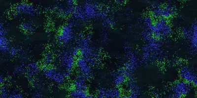
Microbes are rendered in colour and food is rendered in green. For clarity microbes are drawn a little larger than the underlying cell. The simulation supports several colouring schemes: by genome, by age or by energy. There is no limit on how many microbes can occupy a single grid cell; when several are present, their sprites are simply rendered on top of each other at the same position.
 Microbes "live" on a grid that contains randomly distributed food sources.
The simulation runs in discrete time steps. Microbes move along a straight line following their current direction of motion. If the current cell contains food and the microbe's energy is below its maximum, the microbe takes a bite: at most one standard portion per tick, capped by what still fits into its energy reserve and by what is actually still available in the cell. The rest stays put for later ticks or for other microbes. If several microbes share the same cell they eat one after the other from the same supply; whoever runs first in the processing loop eats first.
They are the active part of the simulation and are drawn as small rectangles. They move across the grid and are subject to evolution.
They can move freely into their neighbouring cells along one of eight possible directions of motion. Their current direction is stored as an integer index. This value is used to look up the specific ΔX and ΔY step sizes for the corresponding direction in a small table. Motion is then implemented by adding the delta values to the current grid position of the microbe. The motion table is defined such that only moves into a directly neighbouring cell are possible.
 The eight possible directions of motion of a microbe together with their integer direction index.
| Direction Index | Grid Steps | |
|---|---|---|
| Δx | Δy | |
| 0 | -1 | 1 |
| 1 | 0 | 1 |
| 2 | 1 | 1 |
| 3 | -1 | 0 |
| 4 | 1 | 0 |
| 5 | -1 | -1 |
| 6 | 0 | -1 |
| 7 | 1 | -1 |
At every time step a microbe changes its direction of motion with a certain probability p into one of the seven other possible directions. The eight probabilities for the possible direction changes form the genome of the microbe. The genes are written here as the letter p with an index. The sum of all probabilities is one:
\[\sum_{n=0}^7 p_n = 1\]Each gene corresponds to a segment of the interval [0,1] whose length is proportional to the value of the gene. The following figure shows a randomly drawn genome. Each gene represents the probability of a particular direction change:
To compute the next direction of the microbe given the probabilities stored in its genome, draw a random number \(r\) between 0 and 1:
\[r = rnd(1)\]Then determine the index \(i\) of the gene whose segment contains \(r\). This is the smallest index for which:
\[r \lt \sum_{n=0}^i p_{n}\]In the example above i=3. This is the index of the gene that determines the direction change. The direction \(d\) of the microbe is an integer between 0 and 7, interpreted according to Table 1. The direction at the next time step \(d_{t+1}\) is computed by adding i to the current direction \(d_t\) and taking the remainder modulo 8 (the total number of possible directions):
\[d_{t+1} = (d_{t} + i)\mod 8\]With this equation we can read off the meaning of each gene:
| Gene | Meaning | |
|---|---|---|
| Index i | Identifier | |
| 0 | p0 | No change |
| 1 | p1 | Slight right turn |
| 2 | p2 | Right turn |
| 3 | p3 | Hard right turn |
| 4 | p4 | Reverse |
| 5 | p5 | Hard left turn |
| 6 | p6 | Left turn |
| 7 | p7 | Slight left turn |
 The green arrow marks the microbe's current direction. The cells show the energy cost of each
possible turn. The required energy depends on the magnitude of the direction change. If the
microbe keeps going straight no energy is deducted; a full 180° reverse is the most expensive
manoeuvre at 8 energy points.
The green arrow marks the microbe's current direction. The cells show the energy cost of each
possible turn. The required energy depends on the magnitude of the direction change. If the
microbe keeps going straight no energy is deducted; a full 180° reverse is the most expensive
manoeuvre at 8 energy points.
Each microbe carries a finite energy reserve that it can only increase by eating. In every time step a small portion of that reserve is subtracted as the "basic cost" of staying alive and moving. On top of that, changing direction also costs energy; the sharper the turn, the more is consumed. Only continuous feeding keeps an individual alive: it dies as soon as its energy drops below zero. A microbe that has eaten enough stops taking further bites.
Once an individual has reached a certain age it can, provided it has enough energy, produce offspring. The energy is then split evenly between the parent and the children. The offspring genome is based on the parent genome but contains small random gene variations.
The following table gives an overview of the energy management parameters used in the simulation:
| Parameter | Value |
|---|---|
| Energy gain per food item | 150 |
| Maximum energy | 1500 |
| Reproduction threshold | 1000 |
| Energy lost per tick | 4 |
| Energy lost when changing direction | see steering cost overview |
Each grid cell carries a food reserve between 0 and a hard cap of 255 energy units. Newly spawned food is added to the existing reserve (clipped at 255). On top of that, the reserve of every non-empty cell grows by a small exponential factor each tick (default 1.001/tick). If a cell reaches the cap and still produces food, the surplus spills over into a randomly chosen non-full neighbour cell, so saturated clumps gradually spread into their neighbourhood. Different spawn patterns put the population under evolutionary stress.
On Earth a biome is a large ecological unit defined by a characteristic climate, particular plant and animal communities and typical soil conditions. Tundra, steppe, desert and tropical rainforest are examples. Aquatic biomes such as freshwater and marine ecosystems count too.
In this simulation we simplify that idea drastically: a biome is defined here primarily by the way food is distributed. The biomes differ in both the spatial pattern and the density of the food they generate. How will the simulated creatures respond?
 Biome 1 - Food spawns uniformly in both space and time.
 Biome 2 - Food spawns primarily along horizontal and vertical lines.
 Biome 3 - Food spawns exclusively in a small rectangular area at the centre of the simulation.
 Biome 4 - The wandering circle: a circular spawn field drifts diagonally through the world; static toxic bands flank the drift line.
 Biome 5 - 1000 fixed pair sources of two adjacent cells each continuously generate food.
 Mixed world: a combination of the other biomes. Line grid (left), rectangle (top right) and point sources (bottom right) in a single split arena.
The simulation starts with plenty of food, roughly uniformly distributed, and only a few microbes. Since the genes are set at random it is unlikely that any microbe has a preferred direction of motion. They wander around aimlessly without travelling far from where they started. At the beginning this is not a problem because food is abundant. No matter how clumsy a microbe is, it will probably find enough food to reproduce. The total population grows and suddenly several generations are competing for the same food. The individuals still tend to spin in place, and now the local food supply runs out quickly.
With a uniform food supply the microbes quickly learn to move straight for short bursts.
This lets them reach more distant food sources and escape local competition.
In this situation moving away from the competition is an advantage. Microbes whose genes lead to fewer direction changes suddenly have a competitive edge. They use less energy to stay alive (direction changes are expensive) and they cover longer distances faster, opening up new food sources in the process.
Soon an equilibrium emerges and the population stabilises. Microbes travel long distances in straight lines and only rarely change direction. At this point the population dynamics resemble a classical predator/prey simulation such as the Wator simulation.
The next scenario is referred to in [2] as the "Garden of Eden". Food still spawns randomly across the simulation domain, but there is a small rectangular area at the centre where significantly more food appears. Microbes that reach this region soon show signs of degeneration: they start spinning wildly in tight circles. This behaviour keeps them from leaving the "Garden of Eden", so they stay in the region with the richest food supply.
Food also spawns outside the "Garden of Eden", just at a lower rate. Some microbes adapt and manage to survive there. Food is sparse and they have to cover long distances quickly to stay alive. A second population emerges, with genes optimised for survival in the lean outer region.
The Garden of Eden. Degeneration in the genome of the microbes inside the garden causes
permanent spinning behaviour. Only microbes that fail to leave the Garden of Eden benefit
from its rich food supply.
What happens when you push the "Garden of Eden" idea further can be seen in this biome. Here food spawns almost exclusively along straight horizontal and vertical lines. Between the lines just enough food appears to keep the population from going extinct. At first the microbes fall back on their simplest strategy: they start moving longer stretches in a straight line. Direction changes become rare because they save energy that way and can push out quickly into more distant, untouched parts of the world. This behaviour stays stable for a while.
Food spawns preferentially along lines. After a while a population of line-dwelling
microbes emerges that has almost completely lost the ability to change direction.
Eventually one of the microbes accidentally hits a line and gains a lot of energy in a short time. Its chance of reproducing rises with it. The longer the stretch it covers on the line, the bigger its gain. It will soon leave the line again, but by then it has collected enough energy to produce one or more children. Among those children there may be gene mutations that favour longer straight stretches. Sooner or later another descendant hits a line and the trend reinforces itself more and more.
This scenario was an experiment. The original idea was to demonstrate the use of the reversal gene p4: let a small circular food patch drift diagonally through the world. Anything that stays inside the patch keeps receiving food; anything that leaves it loses access to that food source. The hope was that the microbes would select for the expensive reversal gene p4 in order to match their mean velocity to that of the patch through occasional stochastic direction changes. Two static toxic bands flank the drift line; they penalise sideways escapes and should favour selection of the 180° reverse.
It did not work as expected. In observation it is mostly "cheap turn" strategies — a sequence of several small direction changes — that win out over the expensive 180° reverse. As long as the circle is slow, gentle curves are enough to stay close to it; when it becomes faster the microbes switch to a straight follow strategy and exploit the cyclic 180° flip every 600 ticks to catch the patch again when it returns. The clean reverse demo is therefore the biome with food hotspots. The wandering circle mode is kept in the applet as an experimentation playground.
The wandering circle drifts diagonally through the world; the lateral toxic bands (drawn in
red) should penalise sideways escapes and so favour selection of the 180° reverse. In
practice cheaper multi-turn strategies dominate instead.
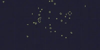
In this scenario food spawns at 1000 fixed pair sources. Each source consists of two directly adjacent grid cells that each emit one standard portion of food per tick. The locations of the sources are randomised on reset but stay constant over a run. Between the sources there is no further food. Anyone who wants to survive has to find one of the sources and stick to it.
The interesting behaviour in this scenario concerns the reversal gene p4. It is normally an expensive, seemingly useless gene that finds practically no use in the other biomes.
A microbe that randomly hits a pair source arrives from one direction. If it tries to continue straight, it leaves the second source cell after a single tick and ends up in the food-poor gap. Zig-zag or gentle-curve strategies leave the source just as quickly. The only moves that keep a microbe at the source for long are drastic reversal manoeuvres. That can be a full 180° reverse, but repeated sharp U-turns in alternating directions can also help.
Point sources scenario. The microbes oscillate by 180° reversals between the two cells of a
source. In the mean genome a clear bar appears in the reverse direction (p4) —
exactly the gene that is consistently selected away in the classical worlds.
In the classical worlds p3, p4 and p5 are the most expensive genes (8 energy units per reverse) and are therefore mutated away. Here it is the other way around: only commuters get access to the full energy stream from a source. Over time a population emerges whose mean genome shows a pronounced bar in the reverse direction or towards sharp turns.
The mixed world combines the previous biomes. The goal was to observe several biomes simultaneously in the same simulation and track how sub-populations evolve in them. The arena is split horizontally into two halves: the left half carries a square line grid like in the line runner biome, the upper right quadrant carries a concentrated food square in the style of the Garden of Eden, and the lower right quadrant is populated with sources as in the hotspot scenario.
The mixed world brings three biomes together in a single arena: line grid (left), Garden of
Eden (top right) and hotspots (bottom right). Three coexisting sub-populations emerge, each
with the genome that works best in its own zone.
Over time several stable sub-populations do indeed emerge side by side, each with the genome that performs best in its respective biome. If you select a subset of microbes from one quadrant via the rubberband drag in the genome panel, the typical fingerprint of that sub-population appears: the left half delivers a line genome dominated by p0, the upper right quadrant a Garden-of-Eden genome with strong turn components, and the lower right quadrant a hotspot genome with a clear p4 bar. Between the zones a handful of generalists wander around — not perfect anywhere, but able to scrape by everywhere.
In principle, and in a very simplified form, this scenario shows the emergence of species adapted to different habitats.
Simulation of a predator/prey model on the toroidal planet Wator.
John Conway's Game of Life — a cellular automaton in which simple rules give rise to complex structures.

The magnetic pendulum simulates the chaotic interaction of a pendulum with three magnets.

The first 3.5 billion years of life on Earth, from chemistry to multicellular organisms.