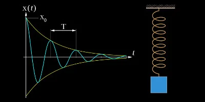
Derivation of the equations of motion of the damped harmonic oscillator with all the details.

In 1994 the German magazine Spektrum der Wissenschaft published an article titled "Experimente zum Chaos" [1] ("Experiments on Chaos"). More than 30 years on, the experimental setup described there is still one of the simplest demonstrations of chaotic behavior. Chaos or chaotic behavior does not, as is often assumed, imply unpredictability in the sense of randomness; it rather denotes a strongly nonlinear sensitivity of an outcome to its initial conditions. The tiniest variation at the start can produce a dramatically different result. As early as 1963, the mathematician and meteorologist Edward Lorenz observed a similar behavior while studying the effect of initial conditions on weather simulations. He wrote:
„One meteorologist remarked that if the theory were correct, one flap of a sea gull's wings would be enough to alter the course of the weather forever. The controversy has not yet been settled, but the most recent evidence seems to favor the sea gulls.“
In later talks the „sea gull" became the more poetic „butterfly", and the term butterfly effect was born.
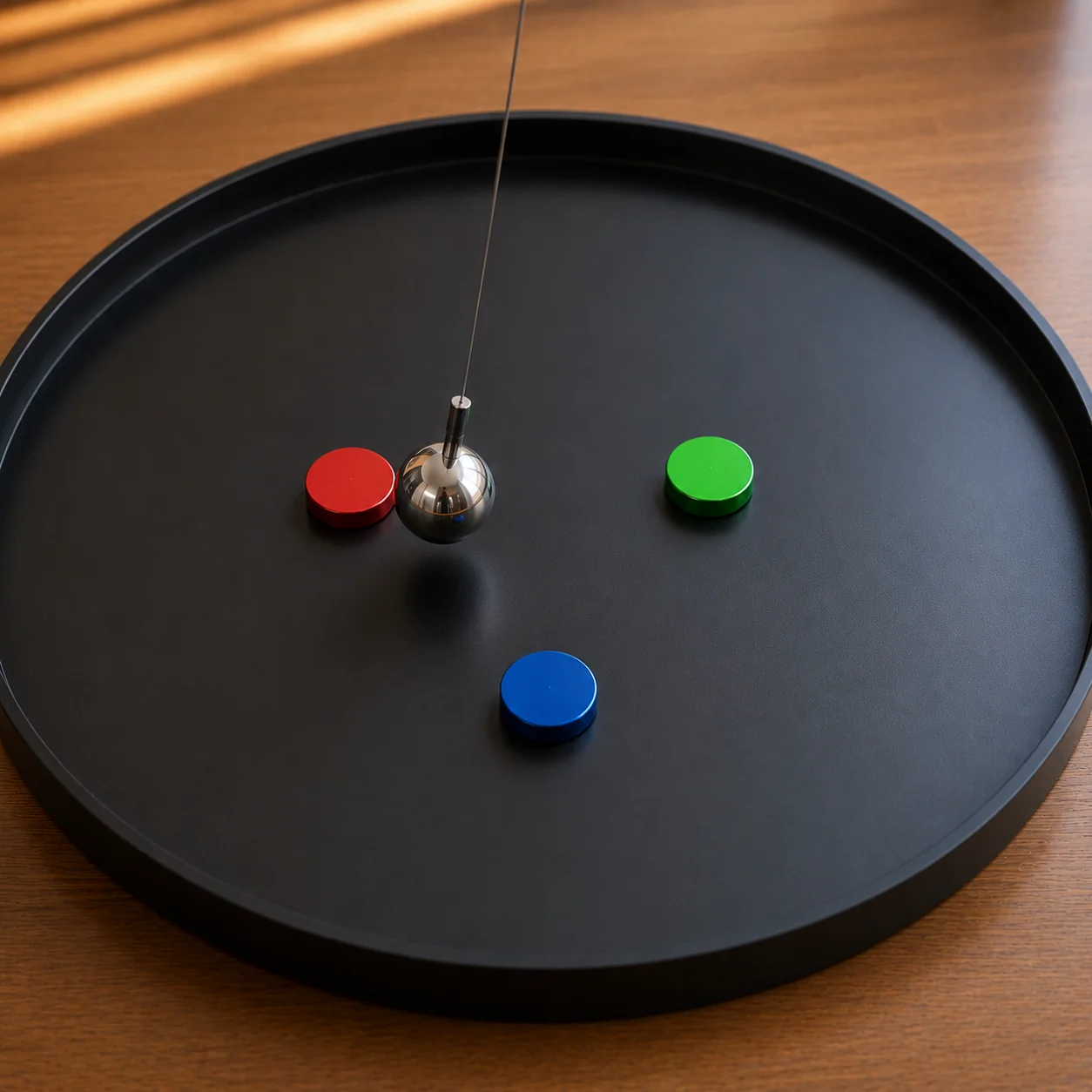 A magnetic pendulum is suspended above three magnets. Once released, it moves under the influence of
the three magnets' attractive force and gravity, which pulls it back towards its rest point.
A magnetic pendulum is suspended above three magnets. Once released, it moves under the influence of
the three magnets' attractive force and gravity, which pulls it back towards its rest point.
The original article describes a simulation of a magnetic pendulum's motion under the influence of gravity and three magnets. A physical setup of the experiment would look like the one shown in image ?. A magnetic pendulum is suspended above three magnets. The magnets are strong enough to keep the pendulum from ever coming to rest in the center position.
Its motion is influenced by friction, gravity and magnetic attraction. The forces are tuned so that the pendulum, losing energy to friction, eventually comes to rest above one of the three magnets. The simulation computes the pendulum's trajectory by integrating the equations of motion of its mass.
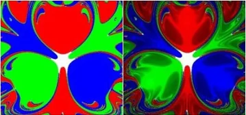
If one colors the starting point of the pendulum's trace with the color of the magnet over which it came to rest, and runs the simulation for a large grid of possible starting positions, a three-colored pattern emerges. It becomes apparent that even small variations in the starting position quickly produce large changes in the pendulum's trajectory. The outcome (the color of the target magnet) thus becomes hard to predict.
Back in 1994 a single simulation run on a supercomputer of that era likely took days. Today you can experience it in high resolution in real time in your browser. The following applet shows the simulation and lets you change the friction strength as well as the positions of pendulum and magnets.
Close to each magnet there are small zones of stability. Releasing the pendulum there makes it settle above the nearest magnet. The farther you move from a magnet, the more chaotic the motion becomes — provided friction is small enough, since at high friction the pendulum quickly comes to rest or simply creeps straight to the nearest magnet.
Less Friction More Friction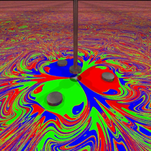 Schematic rendering of the experiment (image courtesy of Paul Nylander).
 Comparison of three different color functions.
In this section I will present the underlying numerical model and show how small changes in the initial conditions of the simulation strongly influence the pendulum's final position. This leads to an inherent unpredictability of the pendulum's endpoint, because the tiniest variation at the start dramatically alters the result.
The classical model assumes a pendulum being attracted by three magnets. Each magnet is assigned a color. The magnets are arranged in an equilateral triangle on a plane below the pendulum, which is suspended centered above them. The magnets are strong enough to prevent the pendulum from ever coming to rest in the center.
The image on the right shows the model schematically. The simulation computes the pendulum's motion under the influence of the three magnets, the restoring force acting on the pendulum, and friction. Because of the energy losses caused by friction, the pendulum will eventually settle above one of the magnets. Its starting point is then colored with that magnet's color. Doing this for every point in the simulation area produces a colored pattern of red, green, and blue pixels.
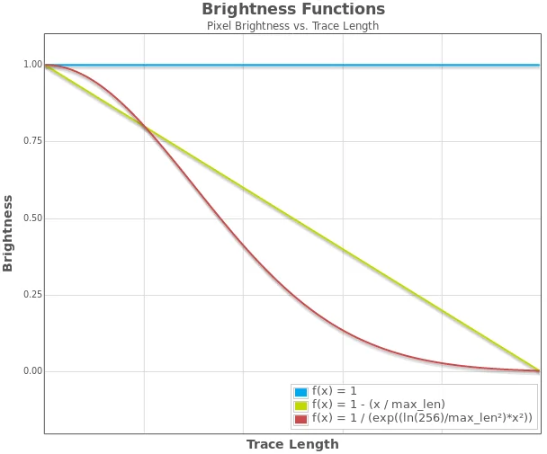
The method described so far only produces three-colored images. It would be desirable to use more colors, or at least shading, in the images. One piece of information available for this is the trace length. A color function based on the trace length is therefore introduced. To simplify scaling, the maximum trace length is taken into account. In principle any function can be used. The functions shown on the right produce good results.
 Darkening colors based on trace length
Starting positions that result in longer traces are rendered in darker shades. The downloadable version of the pendulum simulation allows the use of arbitrary color functions.
If you wonder how the pendulum — with its three spatial dimensions and motion on the surface of a sphere — can be translated into a mathematical model, the answer is: easily! As the saying goes, "if it doesn't fit, make it fit." True to that principle, we simply assume the pendulum is very long. Under this assumption the motion of the pendulum mass can be idealized as motion in a plane above the magnets. For a long pendulum with small deflection one can further assume that the restoring force pulling it back to the center is proportional to the deflection — it then follows Hooke's law. This is extremely convenient, since one can now work in two dimensions without having to worry about torques, rotation angles, cross products and the like.
 Comparison of pendulum restoring force and the attraction caused by the magnets.
Admittedly, it would not have been that much more work to implement the full physics, but reality has a serious drawback once again: the result would have to be mapped onto the surface of a sphere. That would be a little impractical, because, unlike images, you can't hang spheres on a wall nor use them as a desktop background.
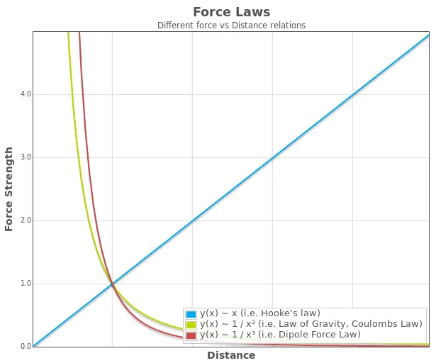
For the calculations we assume that the magnets exert a force on the pendulum that is proportional to the inverse square of the pendulum's distance from the magnet. This is a typical relationship as seen in the law of gravitation or in Coulomb's law. However, this is only half the truth: this force law would only apply if the force were caused by magnetic monopoles, and as far as we know those don't exist. Magnets are always dipoles, and a dipole produces a force that is proportional to 1/r³. This is ignored here, but the curious reader can change it in the configuration file of the downloadable version of the simulation. Furthermore, electrical effects — such as induction and the magnetic fields it produces in the pendulum itself — are neglected.
The pendulum's positions are obtained by integrating the total acceleration acting on it twice. The acceleration follows directly from Newton's second law of motion. The force required to move a body or change its motion equals the product of mass and acceleration. From that the acceleration can be computed directly.
\begin{equation} \nonumber\vec{F} = m \vec{a} \end{equation} \begin{equation} \nonumber\vec{a} = {\vec{F} \over m} \end{equation}Since starting position and initial velocity are given by the initial conditions, all that remains is computing the total acceleration. It is the sum of the accelerations caused by the magnets plus the acceleration caused by the pendulum's restoring force, minus the deceleration caused by friction. For convenience, all further calculations assume a pendulum mass of one mass unit. The following equations result:
Acceleration caused by the restoring force acting on the pendulum:
\begin{equation} \nonumber\vec{a}_g = k_g \cdot \vec{r} \end{equation}Acceleration caused by a single magnet acting on the pendulum:
\begin{equation} \nonumber\vec{a}_m = k_m \cdot \frac{\vec{r}}{|\vec{r}|^3} \end{equation}Deceleration due to friction:
\begin{equation} \nonumber \vec{a}_f = -k_f \cdot \vec{v} \end{equation}Total acceleration of the pendulum:
\begin{equation} \nonumber \vec{a}_t = \vec{a}_g + \Big( \sum_{m=1}^3{\vec{a}_m} \Big) - \vec{a}_f \end{equation}with:
Given a starting position and a starting velocity for the pendulum, a suitable integration scheme can compute the entire trace. This simulation uses the Beeman integration scheme. It is often applied to problems in molecular dynamics and is related to Verlet integration. It is easy to implement and looks as follows in C++:
for (int ct=0; ct<m_nMaxSteps && bRunning; ++ct)
{
  // compute new position
  pos[0] += vel[0]*dt + sqr(dt) * (2.0/3.0 * (*acc)[0] - 1.0 / 6.0 * (*acc_p)[0]);
  pos[1] += vel[1]*dt + sqr(dt) * (2.0/3.0 * (*acc)[1] - 1.0 / 6.0 * (*acc_p)[1]);

  (*acc_n) = 0.0;    // reset accelleration

  // Calculate Force, we deal with Forces proportional
  // to the distance or the inverse square of the distance
  for (std::size_t i=0; i<src_num; ++i)
  {
    const Source &src( m_vSources[i] );
    r = pos - src.pos;
    if (src.type==Source::EType::tpLIN)
    {
      // Hooke's law:          _
      //         _             r         _
      //  m * a = - k * |r| * --- = -k * r
      //                      |r|
      //
      (*acc_n)[0] -= src.mult * r[0];
      (*acc_n)[1] -= src.mult * r[1];
    }
    else
    {
      // Magnet Forces: _
      //      _         r
      //  m * a = k * -----
      //               |r³|
      //
      double dist( sqrt( sqr(src.pos[0] - pos[0]) +
                         sqr(src.pos[1] - pos[1]) +
                         sqr(m_fHeight) ) );
      (*acc_n)[0] -= (src.mult / (dist*dist*dist)) * r[0];
      (*acc_n)[1] -= (src.mult / (dist*dist*dist)) * r[1];
    }

    // Check abort condition
    if (ct>m_nMinSteps && abs(r)<src.size && abs(vel)<m_fAbortVel)
    {
      bRunning = false;
      stop_mag = (int)i;
      break;
    }
  }   // for all sources

  // 3.) Friction proportional to velocity
  (*acc_n)[0] -= vel[0] * m_fFriction;
  (*acc_n)[1] -= vel[1] * m_fFriction;

  // 4.) Beeman integration for velocities
  vel[0] += dt * ( 1.0/3.0 * (*acc_n)[0] + 5.0/6.0 * (*acc)[0] - 1.0/6.0 * (*acc_p)[0] );
  vel[1] += dt * ( 1.0/3.0 * (*acc_n)[1] + 5.0/6.0 * (*acc)[1] - 1.0/6.0 * (*acc_p)[1] );

  // 5.) flip the acc buffer
  tmp = acc_p;
  acc_p = acc;
  acc   = acc_n;
  acc_n = tmp;
}Compiling the source archive requires Visual Studio. A precompiled version is included in the ZIP archive. The program should also run under Linux with Wine. (The animations shown here were created on Linux.)
The C++ sample application is documented in detail here.
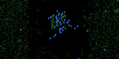
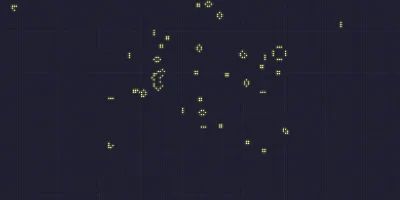
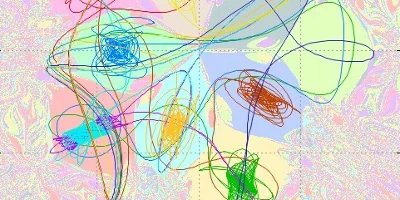
Finally, I would like to present a few images computed with the program shown here. The simulations differ in the number of magnets, their strength, their position, and the pendulum's mount point.
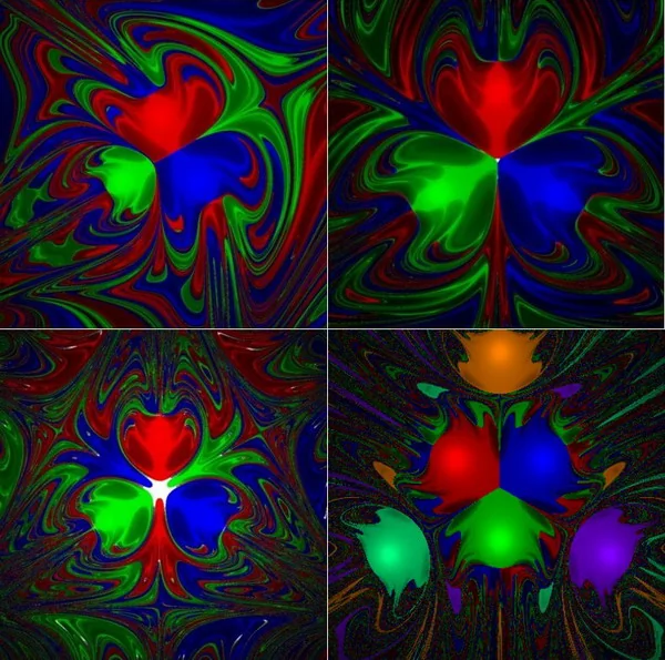 A selection of images computed with different parameters.
Derivation of the equations of motion of the damped harmonic oscillator with all the details.
Simulating a predator-prey model on the toroidal planet Wator.
How simple rules can be used to simulate evolution on a computer.
John Conway's Game of Life is a cellular automaton in which complex structures emerge from simple rules.
Comparing the accuracy of numerical integration schemes — Euler, Runge-Kutta & co. using the magnetic pendulum as a benchmark.