Learn how to write Stellarium scripts with Typescript.

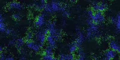
 Simulation of 2D wave equation using finite difference method in Python.
 A page of Python code for solving the wave equation with absorbing boundary conditions. (Click to enlarge)
Today we will learn how to simulate wave propagation in a two-dimensional space using the finite difference method. Mathematically, the wave equation is a hyperbolic partial differential equation of second order. The wave equation looks like this:
\begin{equation} \frac{\partial^2 u}{\partial t^2}(x,y,t) - \alpha^2 \left( \frac{\partial^2 u}{\partial x^2}(x,y,t) + \frac{\partial^2 u}{\partial y^2}(x,y,t) \right) = 0 \label{eq:pde1} \end{equation}It describes how a disturbance of a physical quantity \(u\) moves in time and space in a medium in which waves propagate with velocity \(\alpha\). For this purpose, it combines the second spatial derivatives of the field \(u\) with the second time derivative. What exactly \(u\) is, does not matter. It could stand for a water depth or air pressure. In water, strictly speaking, this equation is only valid for shallow water waves, where the wavelength is much larger than the water depth (e.g. tsunamis).
I do not want to lecture about partial derivatives here, but only present the absolute minimum of that, what is necessary to understand the solution of this differential equation. Equation \(\ref{eq:pde1}\) looks too complicated, so we rewrite it. Fortunately, physicists like operators. An operator is a symbol that stands for one, or a series of operations. For our equation, we need the Laplace operator. It stands for the sum of all the unmixed second partial derivatives in the cartesian coordinates of a field quantity. Furthermore, we use a convention which says that a partial derivative is simply symbolized by subscripts of the quantity to which it is derived. The wave equation then looks like this:
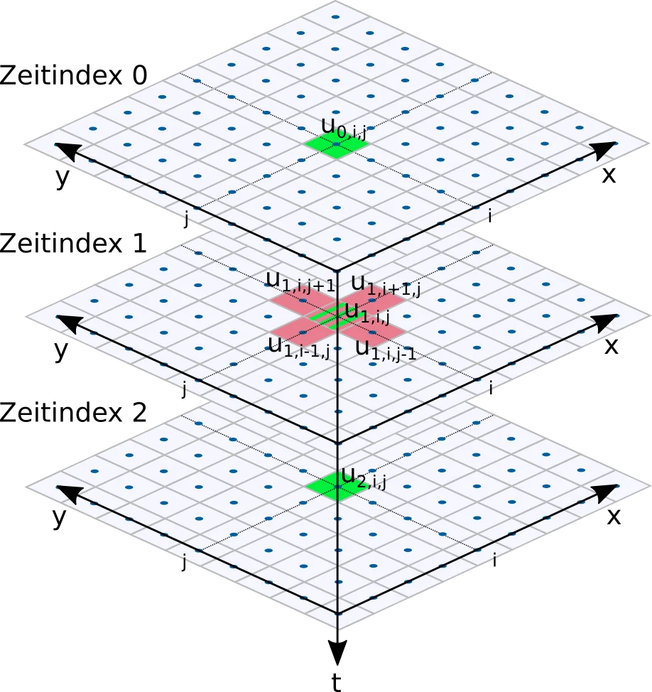 Discretization of the wave equation. Cells needed for the time derivative are colored green, red cells are needed for the Laplace operator.
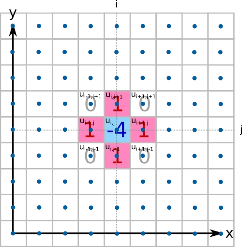 The discrete Laplace operator at the lattice node i,j is calculated from a weighted sum
of the values of the neighboring cells. There are different versions of this operator, which differ in the number of neighboring cells
and their weighting.
\begin{equation}
u_{tt} - \alpha^2 \Delta u = 0 \label{eq:wave2d}
\end{equation}
The discrete Laplace operator at the lattice node i,j is calculated from a weighted sum
of the values of the neighboring cells. There are different versions of this operator, which differ in the number of neighboring cells
and their weighting.
\begin{equation}
u_{tt} - \alpha^2 \Delta u = 0 \label{eq:wave2d}
\end{equation}
This equation is just another form of equation \(\ref{eq:pde1}\). But here it becomes clearer, that we need only two things to solve the differential equation: The second derivative of the field quantity with respect to the time and the result after application of the Laplace operator.
Since we are looking for a numerical solution, we need to discretize the problem. Our simulation domain will be a grid. We need two spatial dimensions and one time dimension. For the time dimension, we are only interested in the current and the two previous time steps.
We need three data arrays that store the state of the physical property at three successive points in time: \(u^{(0)}, u^{(1)}, u^{(2)}\). The time index 0 stands for the future, index 1 represents the current state, and index 2 represents the previous state of the field.
The nodes of the grid have the spatial distance \(h\) from one other and in the time dimension the difference between two computational steps is \(t\). Each of the grid nodes represents an approximate value of the field \(u(x,y)\) at the position \(u(i*h, j*h)\).
Let's start with the computation of the time derivative \(u_{tt}\) at a grid node i,j and time index 1. For the numerical calculation of this derivative we use a 2nd order difference quotient. This requires, in addition to the current value of the field size \(u^{(1)}_{i,j}\), a value from the future \(u^{(0)}_{i,j}\) and one from the past \(u^{(2)}_{i,j}\).
\begin{equation} u^{(1)}_{{tt}_{i,j}} = \frac{u^{(0)}_{i,j} - 2 u^{(1)}_{i,j} + u^{(2)}_{i,j}}{t^2} \label{eq:timediff} \end{equation}Of course, we do not know the value from the future yet. Its computation is the entire point of the finite difference method and we will get to that soon. Beside the second time derivative we still need the Laplace operator for the 2nd spatial derivative in x and y direction.
The discrete version of the two-dimensional Laplace operator \(\mathbf{D}^2_{i,j}\) used here requires the values in the 4 neighboring cells in x and y direction for the calculation. Those will be added to one another and then the value of the field in the node i,j with quadruple weighting is subtracted:
\begin{equation} \quad \mathbf{D}^2_{i,j}=\begin{bmatrix}0 & 1 & 0\\1 & -4 & 1\\0 & 1 & 0\end{bmatrix} \end{equation}The value of the Laplace Operator at grid node i,j can therefore be approximated as:
\begin{equation} \Delta u^{(1)}_{i,j} = \frac{u^{(1)}_{i-1,j}+u^{(1)}_{i+1,j}+u^{(1)}_{i,j-1}+u^{(1)}_{i,j+1} - 4 u^{(1)}_{i,j}}{h^2} \label{eq:laplace} \end{equation}If we now substitute the equations \(\ref{eq:timediff}\) and \(\ref{eq:laplace}\) into equation \(\ref{eq:wave2d}\) then we get a discrete form of the wave equation:
\begin{equation} \frac{u^{(0)}_{i,j} - 2 u^{(1)}_{i,j} + u^{(2)}_{i,j}}{t^2} - \alpha^2 * \left( \frac{u^{(1)}_{i-1,j}+u^{(1)}_{i+1,j}+u^{(1)}_{i,j-1}+u^{(1)}_{i,j+1} - 4 u^{(1)}_{i,j}}{h^2} \right)= 0 \end{equation}Now we solve this equation for \(u^{(0)}_{i,j}\), because we are interested in the field value in the future:
With this equation we can calculate each grid node in \(u^{(0)}\) from the two previous time steps \(u^{(1)}\) and \(u^{(2)}\). To do this, we iterate over all nodes of the field. For this to work we have to specify the values in the fields \(u^{(1)}\) and \(u^{(2)}\) as initial conditions. This method is also known as a second order explicit Euler method.
A simple solution to the wave equation using the finite difference method can be implemented in just a few lines of Python source code. The source code for an example implementation with second-order accuracy in spatial and time dimensions and with static boundary conditions can be found in the waves_2d.py file of the Github archive of this article series.
import pygame
import numpy as np
import random

h = 1        # spatial step width
k = 1        # time step width
dimx = 300   # width of the simulation domain
dimy = 300   # height of the simulation domain
cellsize = 2 # display size of a cell in pixel

def init_simulation():
    u = np.zeros((3, dimx, dimy))         # The three dimensional simulation grid
    c = 0.5                               # The "original" wave propagation speed
    alpha = np.zeros((dimx, dimy))        # wave propagation velocities of the entire simulation domain
    alpha[0:dimx,0:dimy] = ((c*k) / h)**2 # will be set to a constant value of tau
    return u, alpha

def update(u, alpha):
    u[2] = u[1]
    u[1] = u[0]

    # This switch is for educational purposes. The fist implementation is approx 50 times slower in python!
    use_terribly_slow_implementation = False
    if use_terribly_slow_implementation:
        # Version 1: Easy to understand but terribly slow!
        for c in range(1, dimx-1):
            for r in range(1, dimy-1):
                u[0, c, r]  = alpha[c,r] * (u[1, c-1, r] + u[1, c+1, r] + u[1, c, r-1] + u[1, c, r+1] - 4*u[1, c, r])
                u[0, c, r] += 2 * u[1, c, r] - u[2, c, r]
    else:
        # Version 2: Much faster by eliminating loops
        u[0, 1:dimx-1, 1:dimy-1]  = alpha[1:dimx-1, 1:dimy-1] * (u[1, 0:dimx-2, 1:dimy-1] +
                                            u[1, 2:dimx,   1:dimy-1] +
                                            u[1, 1:dimx-1, 0:dimy-2] +
                                            u[1, 1:dimx-1, 2:dimy] - 4*u[1, 1:dimx-1, 1:dimy-1]) \
                                        + 2 * u[1, 1:dimx-1, 1:dimy-1] - u[2, 1:dimx-1, 1:dimy-1]

    # Not part of the wave equation but I need to remove energy from the system.
    # The boundary conditions are closed. Energy cannot leave and the simulation keeps adding energy.
    u[0, 1:dimx-1, 1:dimy-1] *= 0.995

def place_raindrops(u):
    if (random.random()<0.02):
        x = random.randrange(5, dimx-5)
        y = random.randrange(5, dimy-5)
        u[0, x-2:x+2, y-2:y+2] = 120

def main():
    pygame.init()
    display = pygame.display.set_mode((dimx*cellsize, dimy*cellsize))
    pygame.display.set_caption("Solving the 2d Wave Equation")

    u, alpha = init_simulation()
    pixeldata = np.zeros((dimx, dimy, 3), dtype=np.uint8 )

    while True:
        for event in pygame.event.get():
            if event.type == pygame.QUIT:
                pygame.quit()
                return

        place_raindrops(u)
        update(u, alpha)

        pixeldata[1:dimx, 1:dimy, 0] = np.clip(u[0, 1:dimx, 1:dimy] + 128, 0, 255)
        pixeldata[1:dimx, 1:dimy, 1] = np.clip(u[1, 1:dimx, 1:dimy] + 128, 0, 255)
        pixeldata[1:dimx, 1:dimy, 2] = np.clip(u[2, 1:dimx, 1:dimy] + 128, 0, 255)

        surf = pygame.surfarray.make_surface(pixeldata)
        display.blit(pygame.transform.scale(surf, (dimx * cellsize, dimy * cellsize)), (0, 0))
        pygame.display.update()

if __name__ == "__main__":
    main()
This Python script uses the random, numpy and pygame libraries. The libraries numpy and pygame must have been installed via Python's package manager PIP before the program can be executed. After the import statements follows the definition of some global variables. Time as well as location step sizes are defined and two fields are created in the init_simulation function: A three-dimensional field for the field size u (2 spatial dimensions and one time dimension) and a two-dimensional field where the wave propagation velocity within the simulation domain is stored.
In this version of the simulation, the wave propagation velocity is constant throughout the simulation domain. The initial conditions of the field u are 0 in the whole Simulation area. So when the program starts, nothing will happen at first, because the initial wave field is constant zero everywhere. Only after some time "raindrops" will be placed randomly in the function place_raindrops.
import pygame
import numpy as np
import random

h = 1        # spatial step width
k = 1        # time step width
dimx = 300   # width of the simulation domain
dimy = 300   # height of the simulation domain
cellsize = 2 # display size of a cell in pixel

def init_simulation():
    u = np.zeros((3, dimx, dimy))         # The three dimensional simulation grid
    c = 0.5                               # The "original" wave propagation speed
    alpha = np.zeros((dimx, dimy))        # wave propagation velocities of the entire simulation domain
    alpha[0:dimx,0:dimy] = ((c*k) / h)**2 # will be set to a constant value of tau
    return u, alpha
The heart of the simulation is in the update function. This is where the wave equation is solved. At the beginning of the function the fields of the last two time steps are copied over or "moved forward". The field with the index 0 will take the new results. Its state will be copied to the field with time index 1 and the values from there will be moved to time index 2. Older values will be discarded.
def update(u, alpha):
    u[2] = u[1]
    u[1] = u[0]

    # This switch is for educational purposes. The fist implementation is approx 50 times slower in python!
    use_terribly_slow_implementation = False
    if use_terribly_slow_implementation:
        # Version 1: Easy to understand but terribly slow!
        for c in range(1, dimx-1):
            for r in range(1, dimy-1):
                u[0, c, r]  = alpha[c,r] * (u[1, c-1, r] + u[1, c+1, r] + u[1, c, r-1] + u[1, c, r+1] - 4*u[1, c, r])
                u[0, c, r] += 2 * u[1, c, r] - u[2, c, r]
    else:
        # Version 2: Much faster by eliminating loops
        u[0, 1:dimx-1, 1:dimy-1]  = alpha[1:dimx-1, 1:dimy-1] * (u[1, 0:dimx-2, 1:dimy-1] +
                                            u[1, 2:dimx,   1:dimy-1] +
                                            u[1, 1:dimx-1, 0:dimy-2] +
                                            u[1, 1:dimx-1, 2:dimy] - 4*u[1, 1:dimx-1, 1:dimy-1]) \
                                        + 2 * u[1, 1:dimx-1, 1:dimy-1] - u[2, 1:dimx-1, 1:dimy-1]

    # Not part of the wave equation but I need to remove energy from the system.
    # The boundary conditions are closed. Energy cannot leave and the simulation keeps adding energy.
    u[0, 1:dimx-1, 1:dimy-1] *= 0.995
The calculation takes place in only 4 lines of source code. These lines are the direct implementation of equation \(\ref{eq:findiff}\). They work, but make the simulation unbearably slow, because in Python the processing of for-loops is very slow. If you want to reprogram this problem in another programming language, feel free to program with loops. For Python this code has only academic value.
def update(u, alpha):
    for c in range(1, dimx-1):
        for r in range(1, dimy-1):
            u[0, c, r]  = alpha[c,r] * (u[1, c-1, r] + u[1, c+1, r] + u[1, c, r-1] + u[1, c, r+1] - 4*u[1, c, r])
            u[0, c, r] += 2 * u[1, c, r] - u[2, c, r]
For a usable Python version we have to rewrite the source code. We will use a feature called "vectorization". The following code is equivalent to the source code above, but does not use for-loops at all.
	u[0, 1:dimx-1, 1:dimy-1] = alpha[1:dimx-1, 1:dimy-1] * ( \
		u[1, 0:dimx-2, 1:dimy-1] + \
		u[1, 2:dimx,   1:dimy-1] + \
		u[1, 1:dimx-1, 0:dimy-2] + \
		u[1, 1:dimx-1, 2:dimy] - 4*u[1, 1:dimx-1, 1:dimy-1]) \
		+ 2 * u[1, 1:dimx-1, 1:dimy-1] - u[2, 1:dimx-1, 1:dimy-1]
Vectorized operations in Python work with ranges of input vectors. Thus it is possible to avoid the explicit iteration over the the simulation domain. One can calculate thousands of values with a single equation. Where in the first version single cells were computed in a loop now entire index ranges are addressed at once.
With u[0, 1:dimx-1, 1:dimy-1] we address the complete field u, except its boundary area. This is equivalent to using u[0, c, r] in the double loop above. If we want to address u[0,c-1,r], we simply need to subtract the "-1" from the index range of column 1:dimx-1 and write in the vectorized form u[0, 0:dimx-2, 1:dimy-1]. This looks much more complicated, but is orders of magnitude (estimated 50x) faster in execution.
The rest of the program contains the already mentioned function for randomly placing raindrops and the main loop with the code for the visualization. For the visualization of the results, the value of the field u in the three time steps is simply converted to grayscale values and written directly to the output window using pygame.
If you only want to program a water effect, you won't mind that the explicit Euler method is not very accurate. It is by far the easiest method to implement and therefore also the most frequently used in a non academic context. The effect looks realistic at first sight. However, the method has a low error order O(h2). This low error order will cause numerical artifacts especially when using initial conditions with discontinuities in the field. Any wave will almost immidiately be stretched out to an entire wave train. A phenomenon called "numerical dispersion". In reality, a wave crest placed in the center of the grid would diverge into a ring. One would see the ring, nothing else. In our simulation a whole wave train follows the ring.
A simple way to increase computational accuracy is to improve the accuracy of the spatial derivatives computed by the Laplace operator. This can be achieved by the use of a larger discrete Laplace operator. Instead of a version with 3x3 entries (see equation \(\ref{eq:laplace}\)), one can use one with 5x5, 7x7 or even 9x9. The versions of discrete Laplace operators shown here represent higher-order finite difference methods for the spatial derivative [3]:
\(O(h4)\): \begin{equation} \nonumber \mathbf{D}^2_{(i,j)}=\frac{1}{12}\begin{bmatrix}0 & 0 & -1 & 0 & 0\\0 & 0 & 16 & 0 & 0\\-1 & 16 & -60 & 16 & -1\\0 & 0 & 16 & 0 & 0\\0 & 0 & -1 & 0 & 0\end{bmatrix} \end{equation} \(O(h6)\): \begin{equation} \nonumber \mathbf{D}^2_{(i,j)}=\frac{1}{180}\begin{bmatrix}0 & 0 & 0 & 2 & 0 & 0 & 0\\0 & 0 & 0 & -27 & 0 & 0 & 0\\0 & 0 & 0 & 270 & 0 & 0 & 0\\2 & -27 & 270 & -980 & 270 & -27 & 2\\ 0 & 0 & 0 & 270 & 0 & 0 & 0\\ 0 & 0 & 0 & -27 & 0 & 0 & 0\\0 & 0 & 0 & 2 & 0 & 0 & 0\end{bmatrix} \end{equation}A version of the difference equation \(\ref{eq:findiff}\) with a location derivative term of error order 4 looks like this:
The solution of the two-dimensional wave equation using spatial derivatives up to error order 8 is demonstrated in the file waves_2d_improved.py of the accompanying GitHub archive.
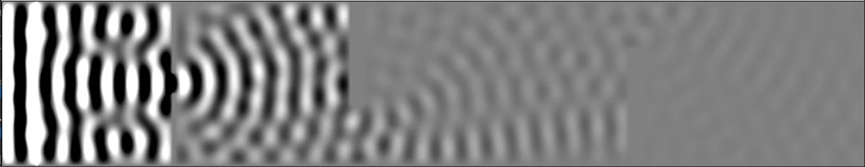
The use of spatial derivatives of higher error order leads to a significant reduction of numerical artifacts, but cannot suppress them completely. The video below shows the comparison of an explicit Euler method with spatial derivative of error order 2 with a method whose spatial derivative has the error order 8 (9x9 Laplace operator). One buys accuracy with higher computational effort, but also reduces the stability of the method. Therefore the maximum possible time step size is a little smaller for methods of higher order.
Numerical solution of the two-dimensional wave equation using an explicit explicit Euler method with spatial derivatives of different error orders.The simulation as described so far has a crucial problem. All waves are reflected at the edge. The energy cannot leave the simulation domain. After a short time the simulated wave tank is filled with waves and you will not be able to see anything other than waves all over the place.
A 3x3 Laplace operator always needs a value in all directions next to the grid point to be calculated. For this reason, it cannot be applied to grid points directly on the edge itself. So far we have therefore fixed the boundary values to a value of 0. These are so-called Dirichlet boundary conditions. Therefore no energy can be transferred to the outside. This is why all outgoing waves are reflected back.
To simulate an open boundary, we need to solve special differential equations on the boundary. Such conditions are also called "radiating", "absorbing" (ABC) or "Mur boundary conditions" ([4] and [5]). With radiating boundary conditions, the following differential equations apply at the ends of the simulation domain in X-direction:
\begin{align} \frac{\partial u}{\partial x} \biggr\rvert_{x=0} &= -\frac{1}{c} \frac{\partial u}{\partial t} \label{eq:mur1} \nonumber\\ \frac{\partial u}{\partial x}\biggr\rvert_{x=N} &= \frac{1}{c} \frac{\partial u}{\partial t} \label{eq:mur2} \end{align}Analogous equations apply in Y-direction. This results in the following equations for the edges x=0, x=N, y=0 and y=N:
where N is the index of the last grid node. \(\kappa\) is calculated as follows:
\begin{equation} \kappa = \alpha \frac{t}{h} \end{equation}These difference equations are applied to all grid points on the boundary. When using a larger discrete Laplace operator (5x5, 7x7, or 9x9), the boundary region must be chosen wider to include all grid nodes that the Laplace operator cannot cover. The implementation of radiating boundary conditions according to Mur is demonstrated in the file waves_2d_improved.py of the accompanying GitHub archive.
Learn how to write Stellarium scripts with Typescript.
Learn about predator-prey-interactions in the toroidal world of Wator.
How to create animations of the night sky with Python and Stellarium automation.
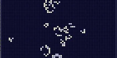
An implementation of John Conway's Game of Life in Python.