Learn about predator-prey-interactions in the toroidal world of Wator.

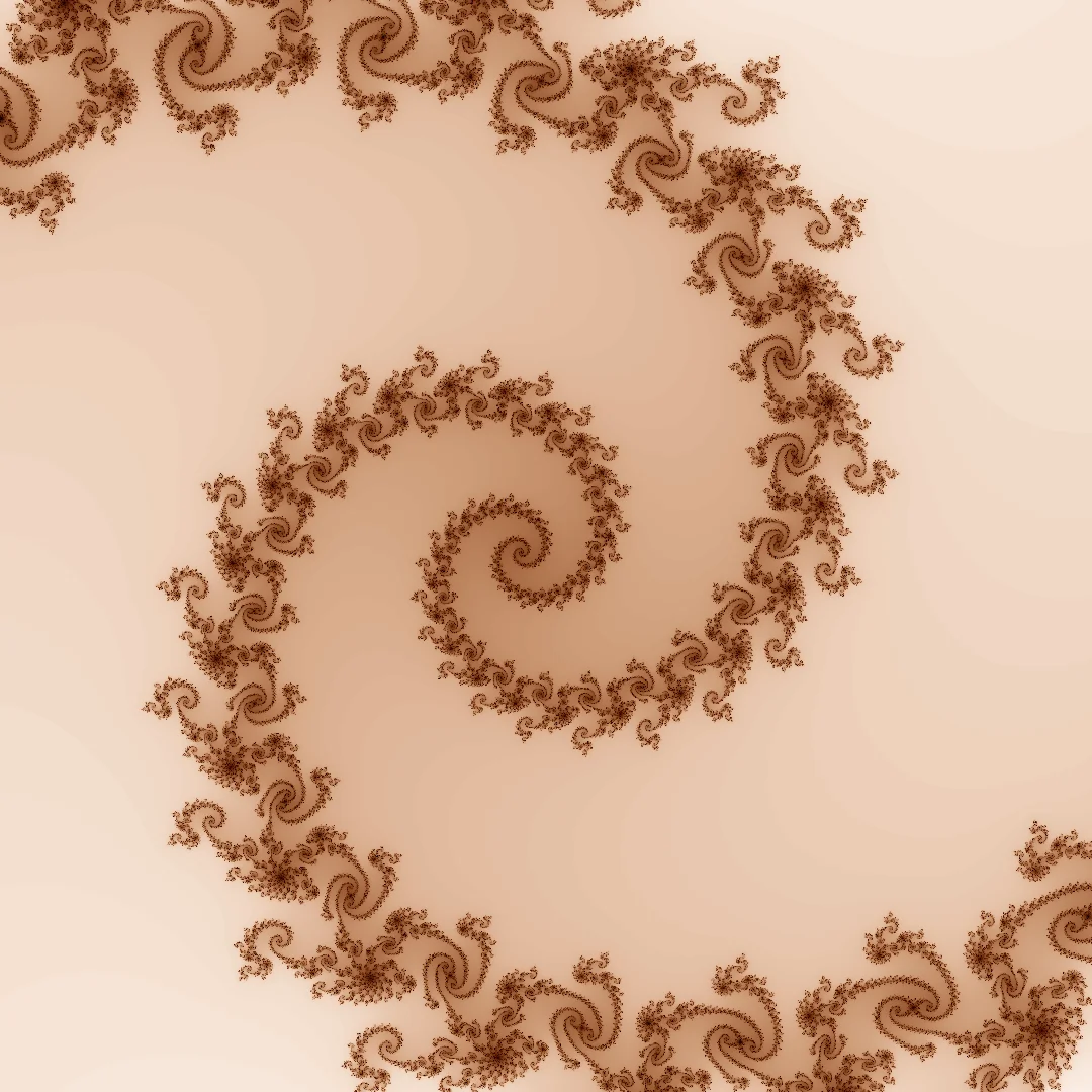
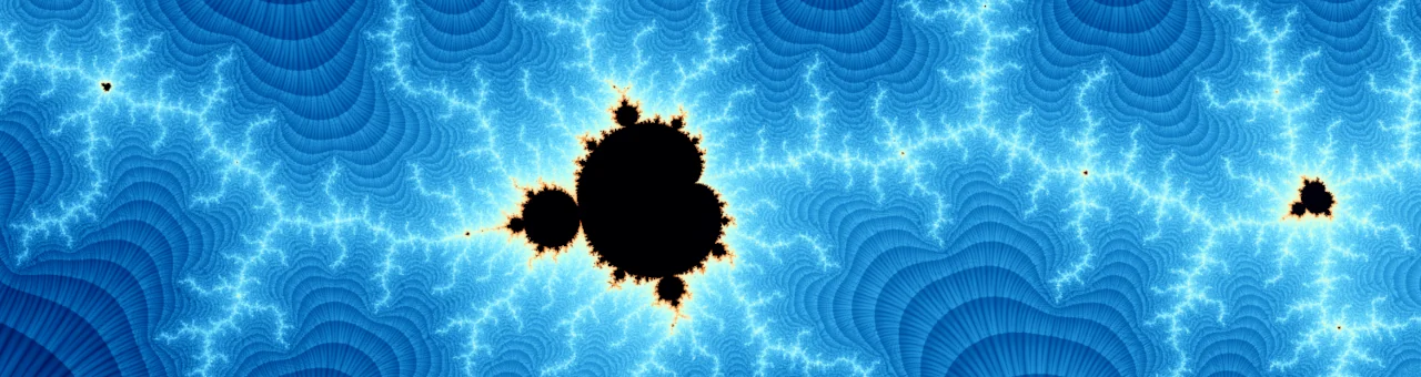 Zooming into the Mandelbrot set reveals ever more copies of the set itself. This self-similarity is a characteristic of fractals.
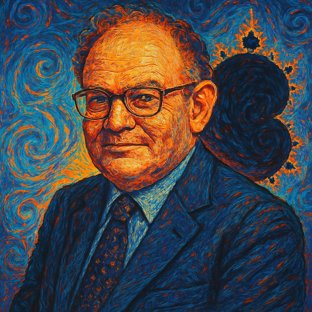 Benoît B. Mandelbrot, the father of fractal geometry. (Portrait generated with AI; OpenAI/Dall-E)
Benoît B. Mandelbrot (20 November 1924 - 14 October 2010) was a French-American mathematician (picture?). He spent most of his working life at the Thomas J. Watson Research Center, the headquarters of IBM's research division. He coined the term "fractal" and discovered the Mandelbrot set, named after him. This number set forms a fractal geometric structure. It is generated by examining the members of the complex-valued series starting with:
\begin{equation} z_0 = 0 \end{equation}and the generating function:
\begin{equation} z_{n+1} = z_n^2 + c \label{eq:formel_mandelbrot} \end{equation}Complex numbers are an extension of the real numbers. They consist of a real part and an imaginary part and are represented in the form z = a + bi, where i is the so-called imaginary unit. A complex number thus represents a point in the complex plane, formed by the real axis and the imaginary axis. Visually, a complex number represents a vector from the origin (0,0) to the point (a,b) in the complex plane. The real part a is the projection of the vector onto the real axis and the imaginary part b is the projection onto the imaginary axis.
The numbers in the complex plane for which the series does not diverge are part of the Mandelbrot set. All other numbers do not belong to this set. The amazing thing about the set is that although the formula for forming it is very simple, the boundary between the elements of the Mandelbrot set and the non-elements forms a very complicated structure. The set has therefore been described as one of the most complex objects in mathematics [1a]. Benoît Mandelbrot himself called such structures fractals.
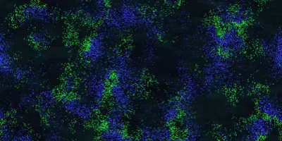
Another characteristic of fractal structures is their self-similarity. No matter what scale you examine them on, you will always find similar shapes. Fractals are often based on a set of simple rules, but lead to an incredible variety of shapes. This self-similarity is also a characteristic found in nature since the beginning of life, and the study of fractals has contributed to a better understanding of the formation and growth processes in nature. The Mandelbrot set is an example of this property and was the catalyst for the popularisation of fractal geometry in the 1980s.
The complex series, which is formed using the formula \(\ref{eq:formel_mandelbrot}\), is called an orbit. By calculating the number of iterations needed to determine whether the series converges or diverges for each point in the complex plane within the range -2 to 2 on the real axis and -1.5 to 1.5 on the imaginary axis, you obtain the following image. By moving the mouse over the image, the orbits of the start point corresponding to the mouse position are displayed in yellow.
The closer one gets to the edge of the Mandelbrot set, the more iterations are necessary to determine whether a point diverges or not. However, it is mathematically proven that the sequence must diverge if a number in the path exceeds an absolute value of 2. With this knowledge, a lot of time can be saved in computations outside the set.
Points that do not diverge are part of the Mandelbrot set and are shown in black. A large number of iterations are required to visually resolve the boundary region. Deciding whether a point is part of the set takes longer the deeper you zoom into the set. While an overview image can be computed with 250 iterations, thousands of iterations are needed for high-resolution detail images.
 Mandelbrot Set after one iteration.
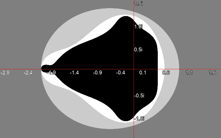 Mandelbrot Set after three iterations.
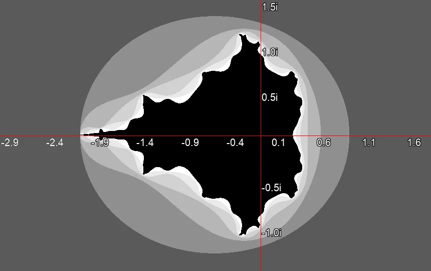 Mandelbrot Set after six iterations.
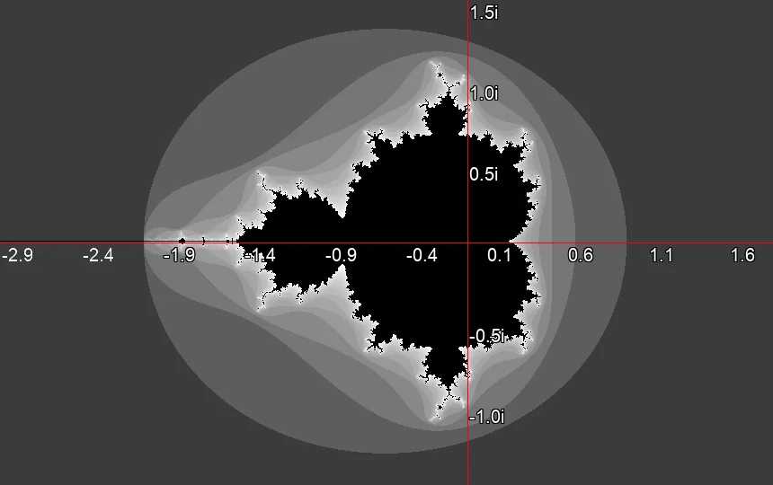 Mandelbrot Set after 19 iterations.
The Mandelbrot Set is connected [4]. The area where the sequence converges, namely the interior of the set, forms no islands. Everything within is connected by thin filaments. The boundary area is very complex and contains many interesting structures (Image ?), which only become visible when zooming in.
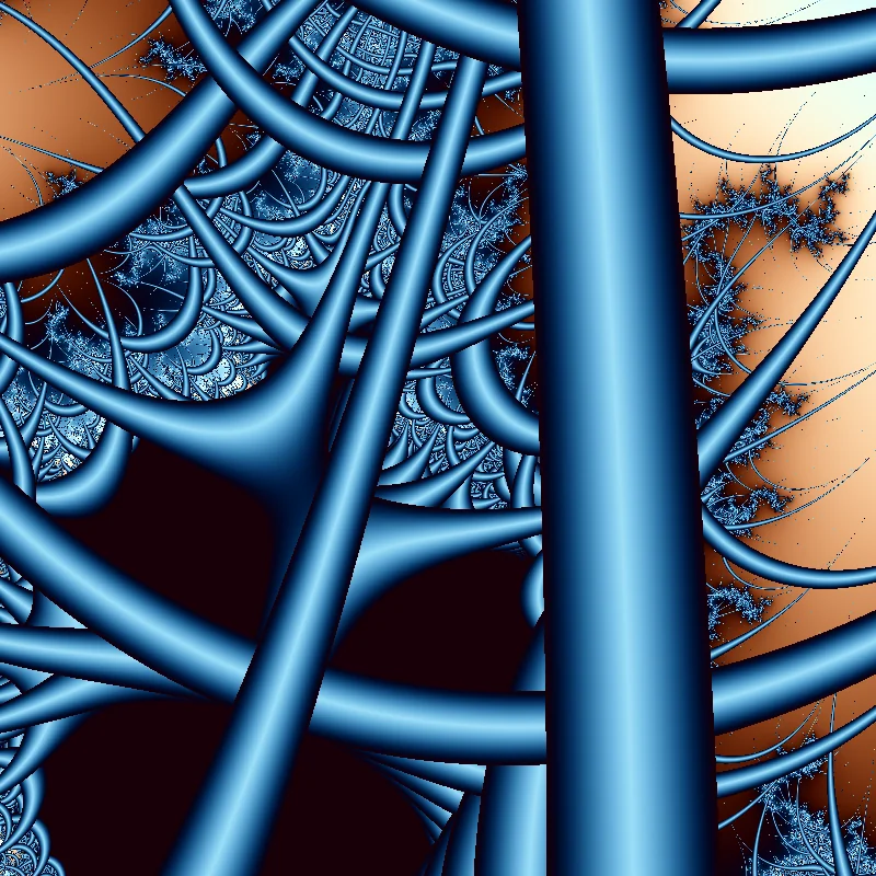
 The edge of the Mandelbrot Set is full of complex structures.
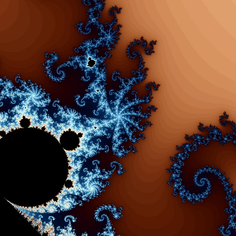 Zooming in reveals ever new, fine structures and spirals.
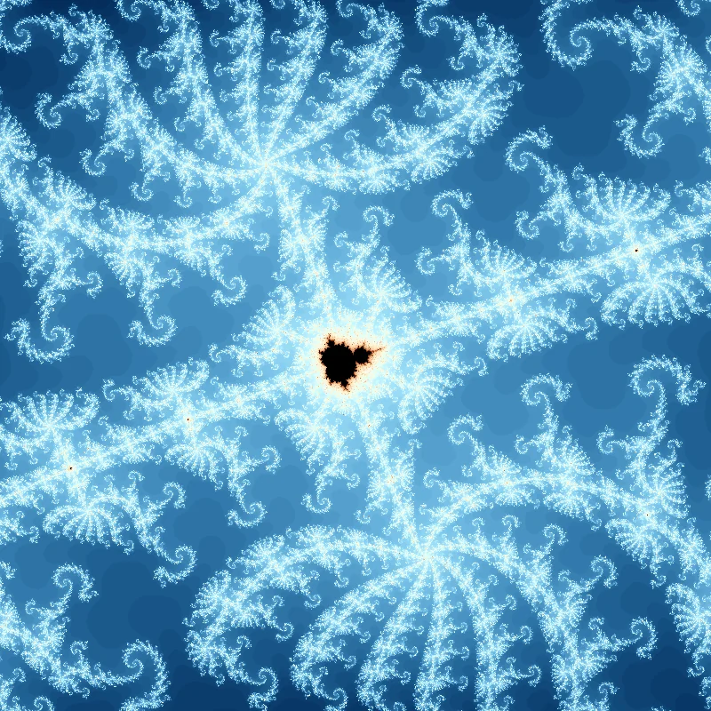 Repeatedly, smaller copies of the Mandelbrot Set appear as well.
You find whirls, spirals (Image ?) and ever again smaller copies of the set itself (Image ?). It is a world full of wonderful details, endlessly recurring in ever-new variations, only limited by computiational power. Because ultimately, infinitely many iterations would be necessary to fully calculate the Mandelbrot set.
The choice of colors has a crucial impact on the representation of the Mandelbrot set. Since its discovery, a variety of increasingly artistic color schemes have been developed.
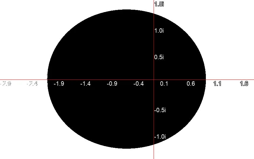
The first representations of the Mandelbrot set were black-and-white and showed, as in Image ? only the points that belonged to the set in black color. This was originally due to the limited capabilities of computers at the time, as the output often occurred on paper or monochrome monitors. Even today, most representations of the Mandelbrot fractal show the set itself only as a black area. Typically, only the pixels that do not belong to the set, whose associated orbits are divergent, are colored.
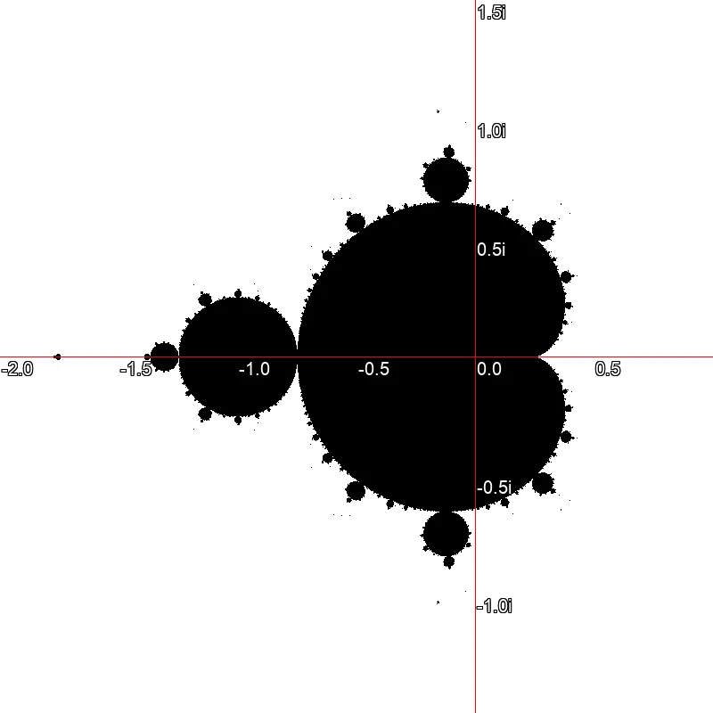 Black and white representation of the Mandelbrot set. The black pixels belong to the set, the white pixels do not.
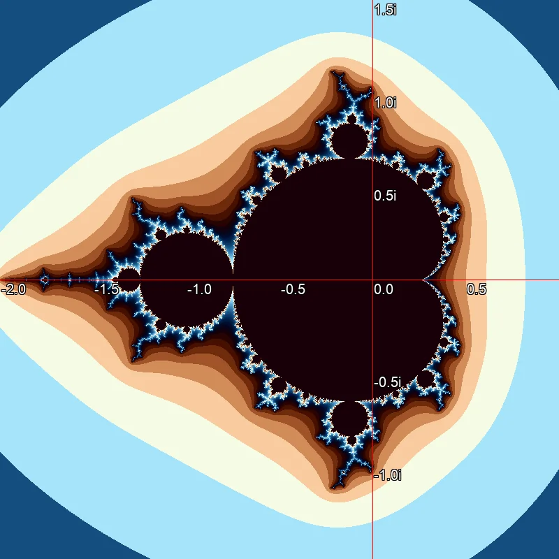 With coloring based on the logarithm of the iteration counter, band-like transitions appear. This is because the number of iterations is an integer.
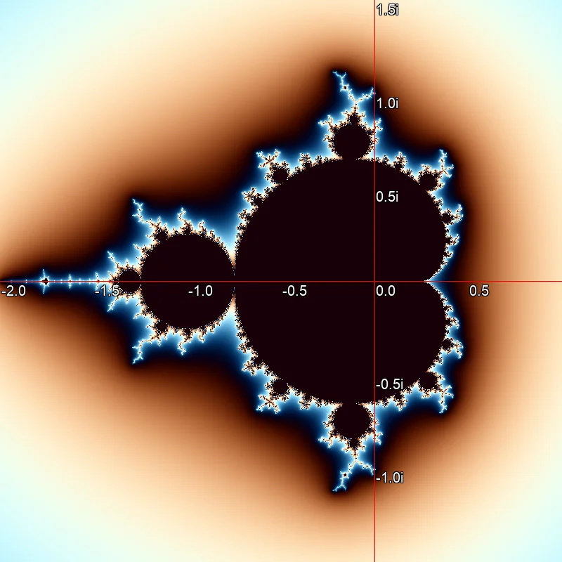 Continuous coloring according to the algorithm described by Linas Vepstas.[2].
With the advent of home computers in the 1980s, it became common to count the number of iterations performed and convert this value into a color using color tables. Later, as computer graphics improved, the logarithm of the iteration counter was calculated and converted into an R,G,B value using formulas, as shown in Image ?. In the 1990s, a method became popular which made it possible to continuously calculate the colors of the Mandelbrot set, as shown in Image ? [2]. This method produces the most beautiful results and was used in the most images shown here. The so-called Smooth-Iteration-Count is calculated using the following formula:
\begin{equation} v = n + 1 - \frac{\log(\log(|z_n|))}{\log(2)} \end{equation}
where:
When calculating the Mandelbrot set, a sequence of numbers, called the orbit, is calculated for each point on the complex plane. Another way to make the fractals more interesting involves the use of what are called Orbit Traps. These are, in the simplest case, geometric shapes placed on the complex plane. The distance to these shapes is measured for each point on an orbit. This value is then used as a criterion for coloring or even for an early termination of the iteration. As these structures terminate the iteration on contact, they are known as Orbit Traps. Simple Orbit Traps might include the real and imaginary axes themselves, the coordinate origin, a unit circle, or arbitrarily placed points.
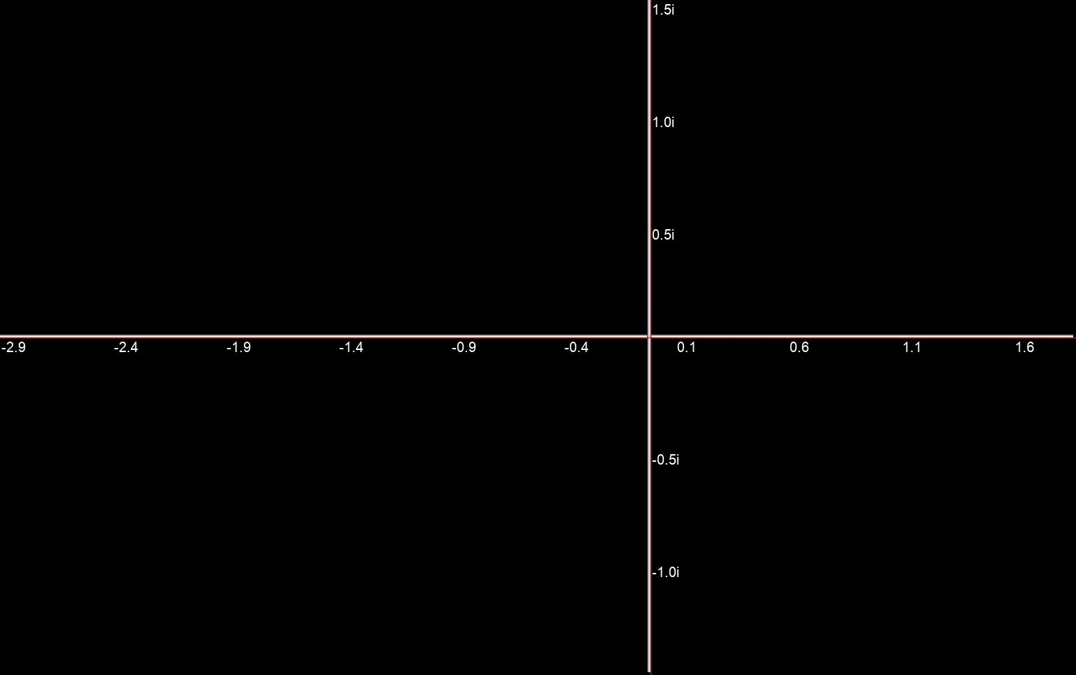 Real and imaginary axes as geometric Orbit Traps.
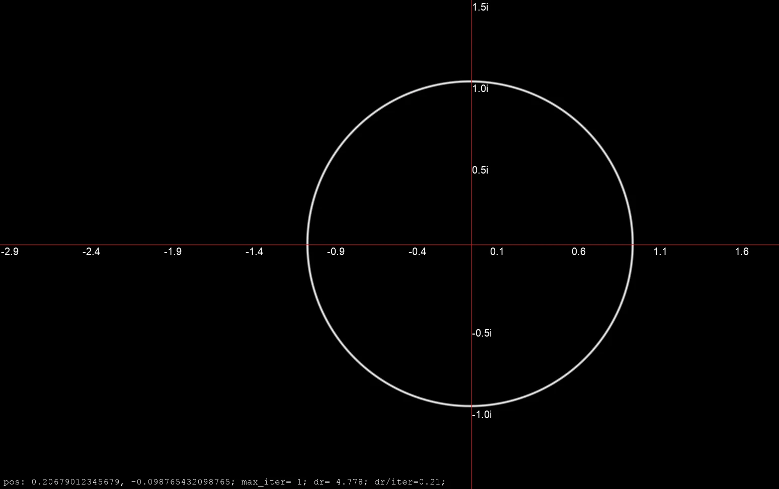 Unit circle as a geometric Orbit Trap.
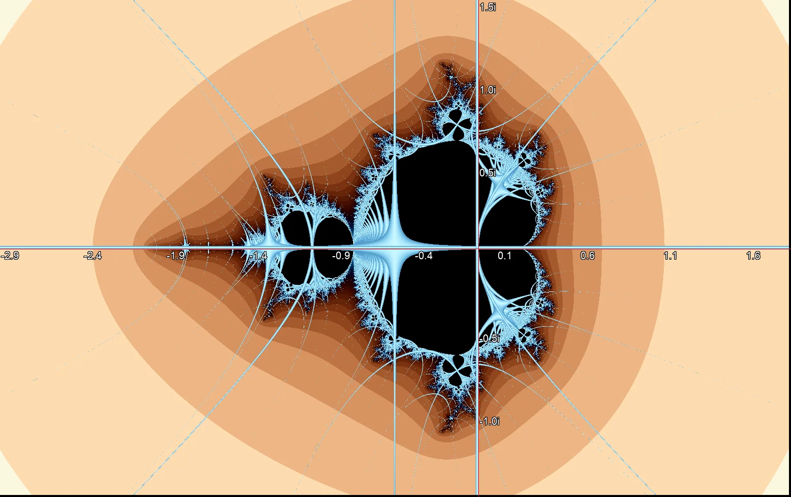 Mandelbrot rendering with real and imaginary axes as geometric Orbit Traps.
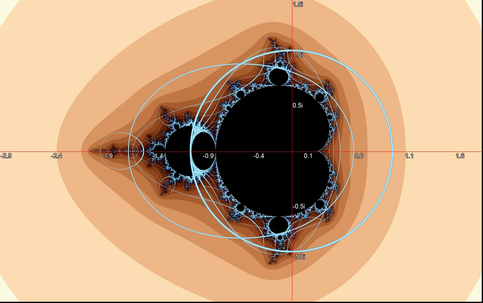 Mandelbrot rendering with the unit circle as a geometric Orbit Trap.
The following source code example shows the main loop of the implementation of a geometric Orbit Trap in Python. The trap is a combination of a circle and the axes of the complex plane. The result is shown in Image ?. Only the result of iteration termination due to contact with the Orbit Trap is drawn. The outlines of the Mandelbrot set are just visible in the background.
 Rendering of a geometric orbit trap, formed by the axes of the complex plane and a circle with radius 0.27 around the coordinate origin.
def compute_mandelbrot(dimx : int, dimy : int,
	maxiter : int, rmin : float, rmax : float, imin : float, imax : float):
    istep = (imax - imin) / dimy
    rstep = (rmax - rmin) / dimx
    mandelbrot_set = np.zeros((dimy, dimx), dtype=np.float64)

    for row in range(dimy):
        for col in range(dimx):
            z = 0
            c = (rmin + col * rstep) + 1j * (imin + row * istep)

            trapped = False
            trap_size = 0.025
            trap_dist = 0
            trap_radius = 0.27
            for k in range(maxiter):
                z = z*z + c

                # circular orbit trap
                if (trap_radius-trap_size) < abs(z) < (trap_radius + trap_size):
                    trap_dist = abs(trap_radius - abs(z))
                    trapped = True

                # real axis trap
                if abs(z.real) < trap_size:
                    trap_dist = abs(z.real)
                    trapped = True

                # imaginary axis trap
                if abs(z.imag) < trap_size:
                    trap_dist = abs(z.imag)
                    trapped = True

                if abs(z) > 2 or trapped:
                    break

            mandelbrot_set[row, col] = 0 if not trapped else trap_dist

return mandelbrot_set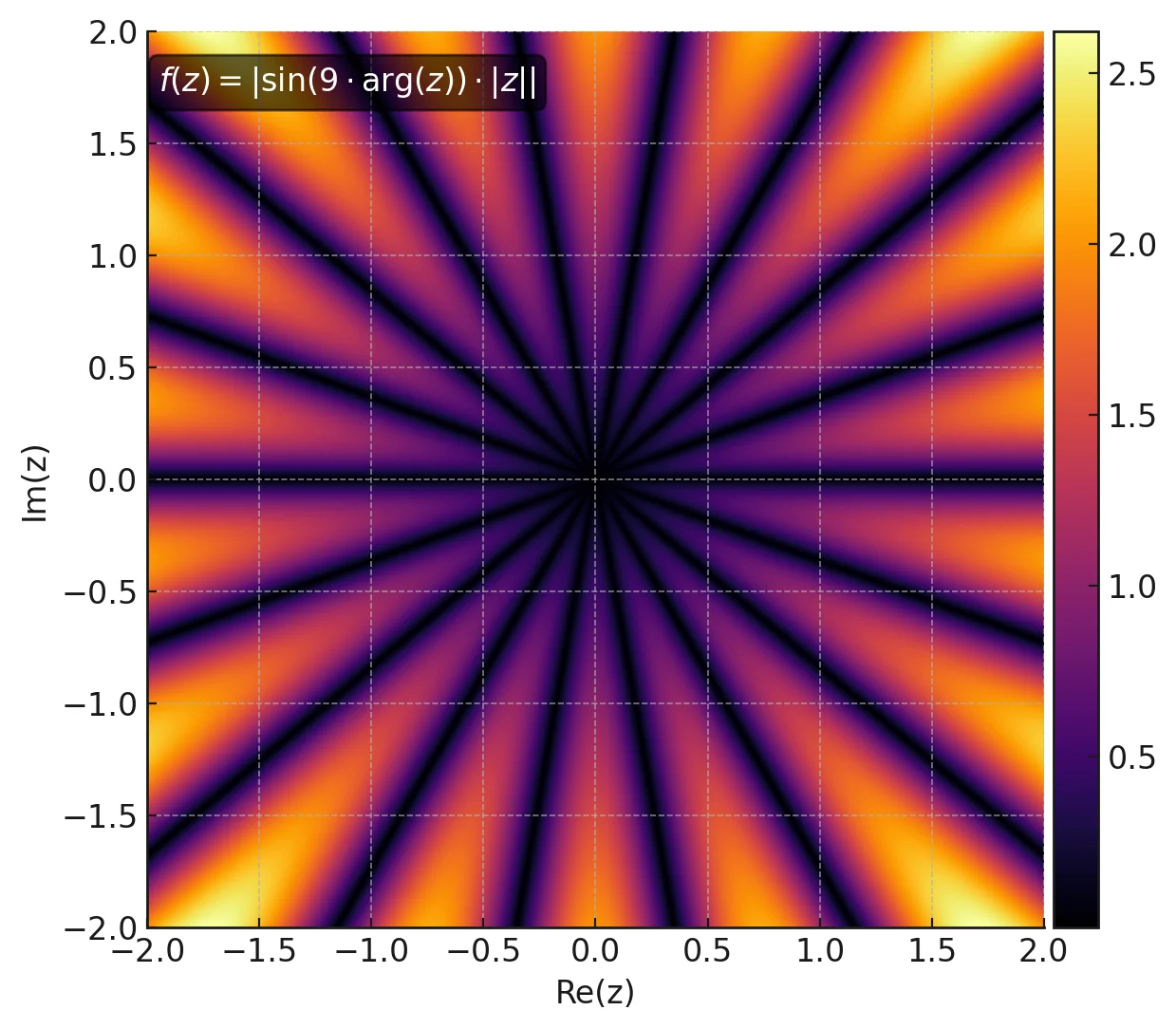 The image shows a petal-shaped orbit trap function with 18-fold angular symmetry.
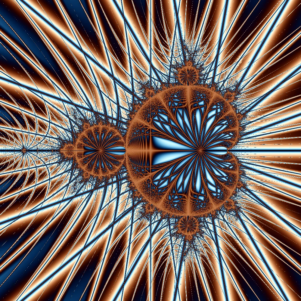
Two-dimensional functions \( f : \mathbb{C} \to \mathbb{R} \) or even images can also be used as orbit traps. Here, the minimal value \(d_{\text{trap}}\) of the function \( f(z_n) \) along all points of the orbit is taken as the criterion for coloration. Alternatively, the trap distance \(d_{\text{trap}}\) could also be used as an additional criterion for iteration termination. The following Mandelbrot images use the orbit trap function shown in Image ?:
\begin{equation} \label{eq:trap_function} f : \mathbb{C} \to \mathbb{R}, \quad f(z) = \left| \sin\left(9 \cdot \arg(z)\right) \cdot |z| \right| \end{equation}The "trap distance" of an orbit then results from:
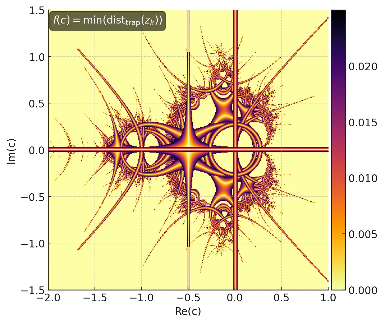
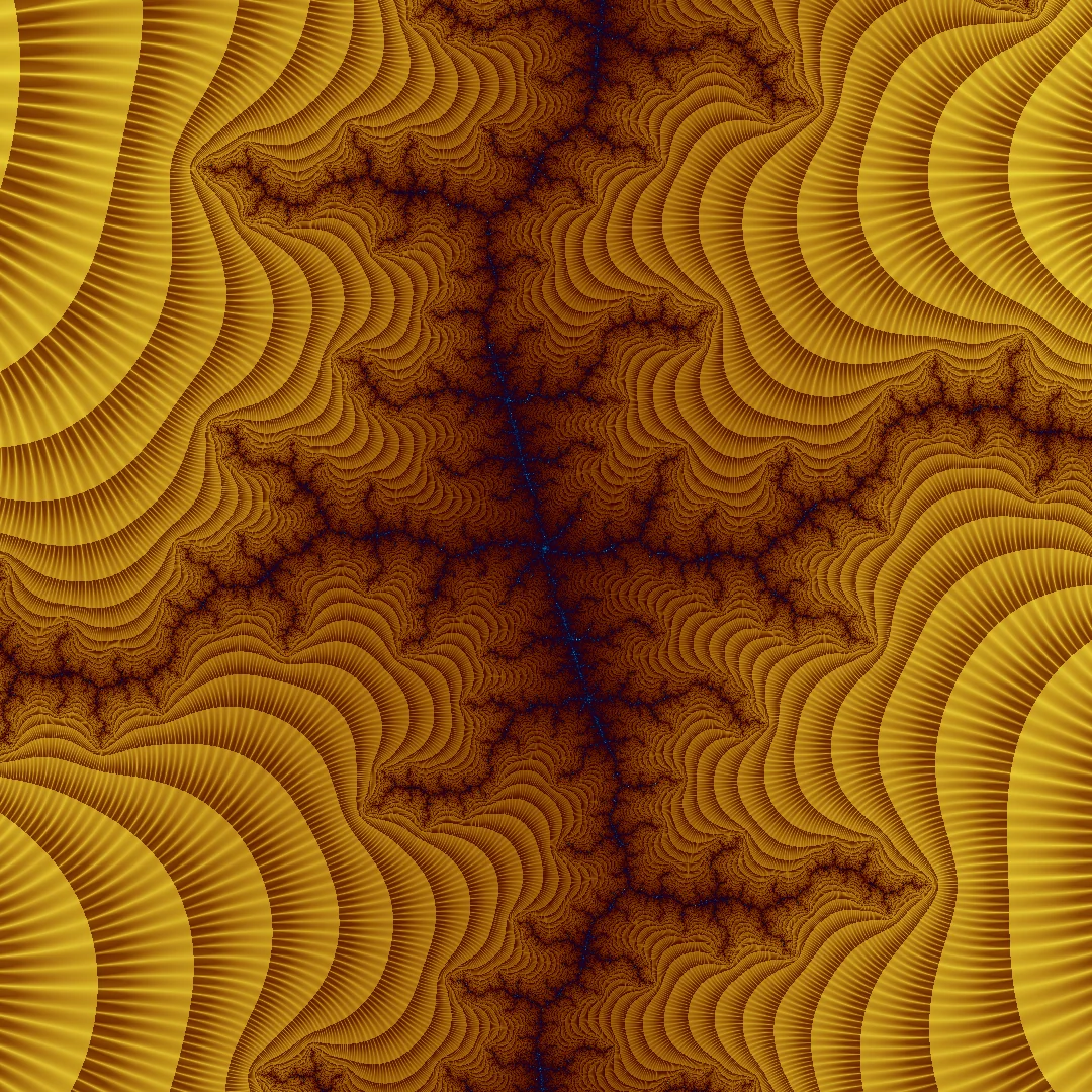
\begin{equation} \label{eq:trap_color} d_{\text{trap}} = \min_n f(z_n) = \min_n \left| \sin\left(9 \cdot \arg(z_n)\right) \cdot |z_n| \right| \end{equation}Now one can choose whether the trap should act only in the core area of the fractal, i.e., the elements of the set itself (Image ?), or over the entire complex plane (Image ?). Geometric orbit traps often create organically appearing structures. Zooming into the fractal then results in three-dimensional looking patterns.
 Mandelbrot with a rosette-shaped orbit trap. The trap only affects the coloration of the elements of the Mandelbrot set itself. Instead of
coloring the points black, the distance to the trap is used as a criterion for coloring. The boundary area is colored using the Smooth Iteration Count as usual.
Mandelbrot with a rosette-shaped orbit trap. The trap only affects the coloration of the elements of the Mandelbrot set itself. Instead of
coloring the points black, the distance to the trap is used as a criterion for coloring. The boundary area is colored using the Smooth Iteration Count as usual.
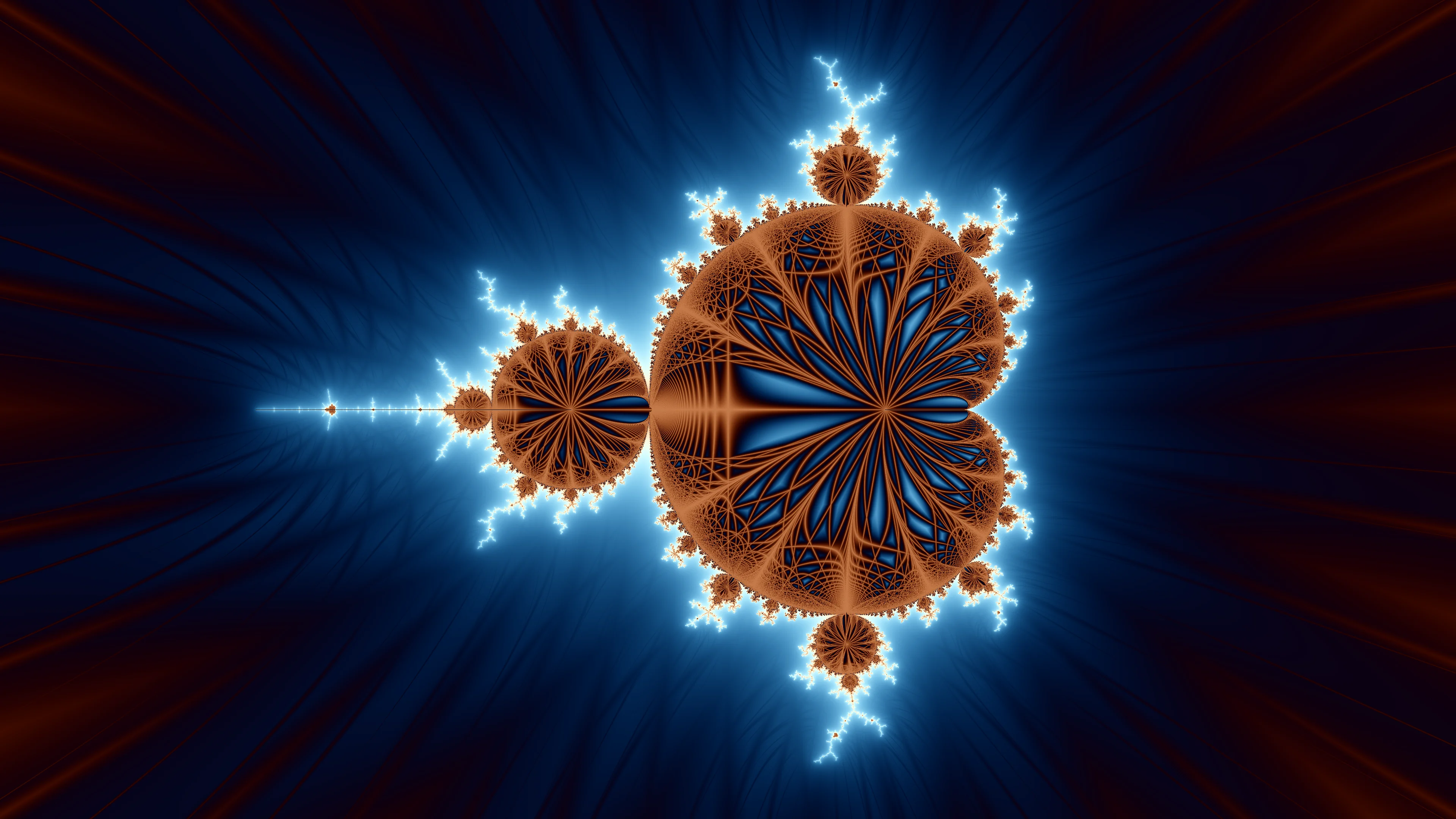
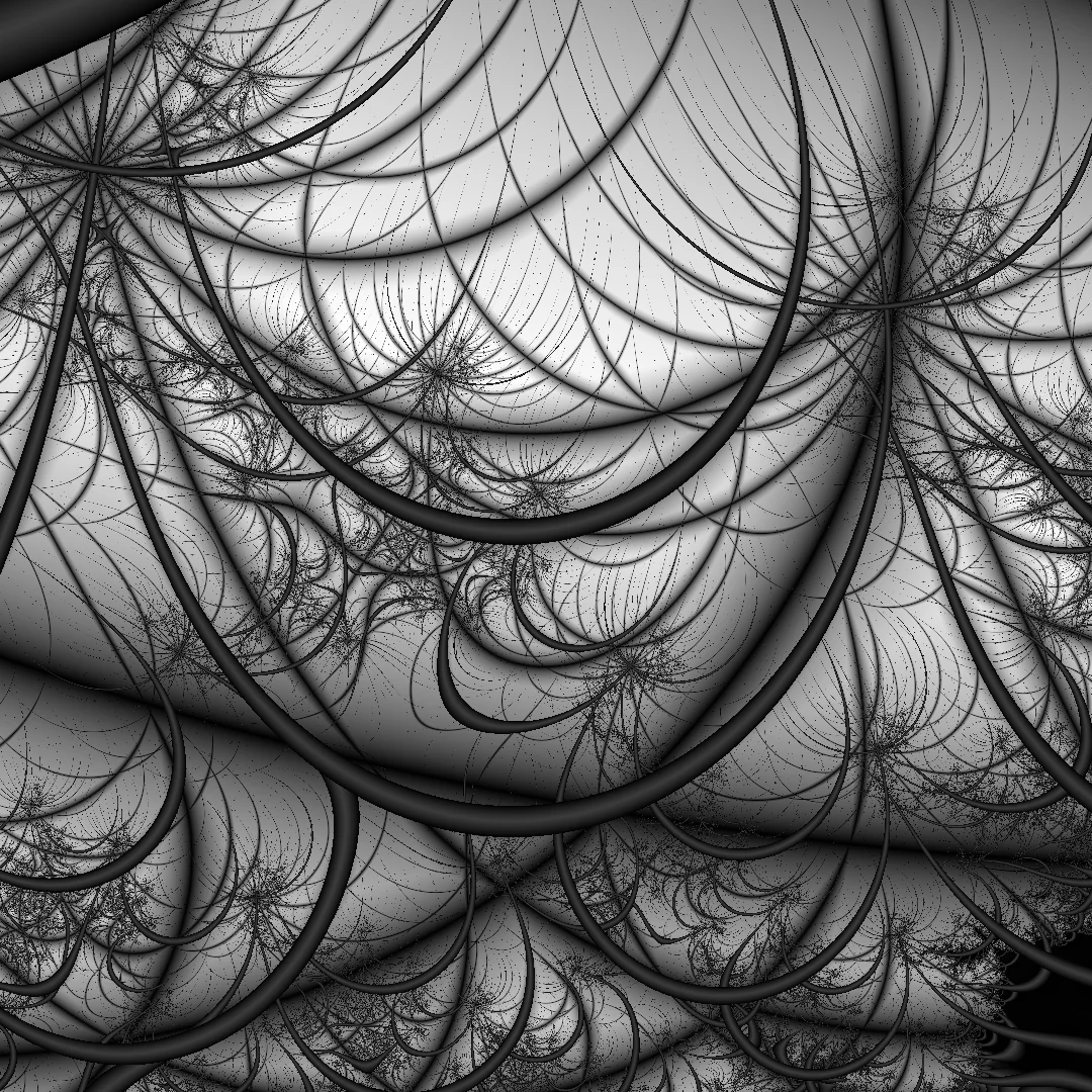
 Here, the same rosette-shaped orbit trap is used. Instead of the number of iterations, however, for all
points on the complex plane, the distance to the trap is used as the criterion for coloration. The iterations
are performed as usual, but the number of iterations is no longer used for coloration.
Here, the same rosette-shaped orbit trap is used. Instead of the number of iterations, however, for all
points on the complex plane, the distance to the trap is used as the criterion for coloration. The iterations
are performed as usual, but the number of iterations is no longer used for coloration.
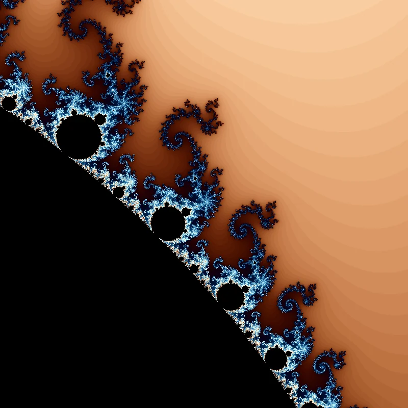
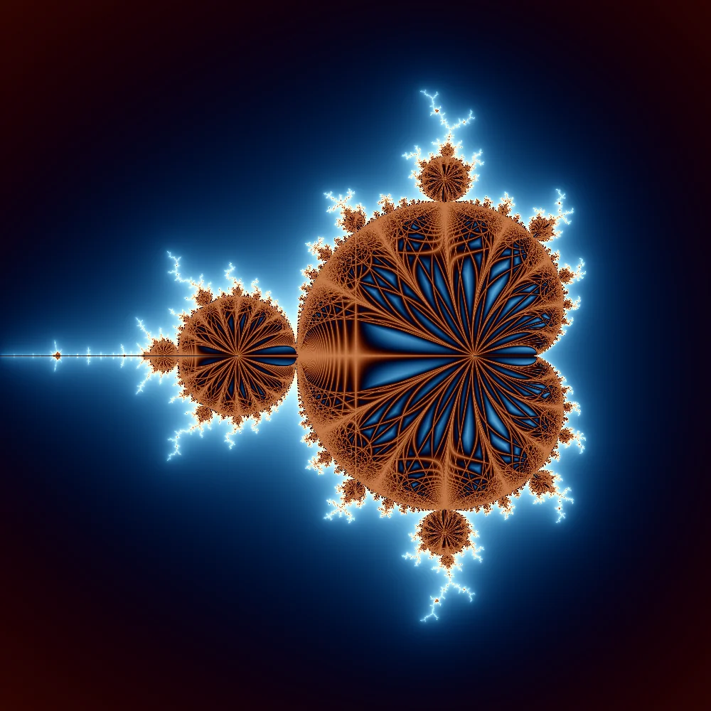
Finally, here is a simple example of calculating a Mandelbrot set with an orbit trap and continuous coloring. Implemented in Python using the Pygame library and Numba, a "Just-in-Time" compiler. The example is designed to be easily adaptable to one's own needs.
 Mandelbrot set with a rosette-shaped orbit trap and continuous iteration counter.
The code example uses the function shown in Figure ?: \[ f : \mathbb{C} \to \mathbb{R}, \quad f(z) = \left| \sin\left(9 \cdot \arg(z)\right) \cdot |z| \right| \] as an orbit trap. The result of calculating the minimal value of this function for the complex values \( z_n \) of an orbit determines the coloring of the elements in the Mandelbrot set. Additionally, this value, slightly scaled down, is added to the value of the continuous iteration counter in the outer area. This reveals the structures of the orbit trap also in the outer area of the fractal.
import pygame
import numpy as np
from numba import jit


@jit
def trap_function(z, petals=5):
    return abs(np.sin(petals * np.angle(z)) * np.abs(z))


@jit
def compute_mandelbrot(dimx : int, dimy : int, maxiter : int, rmin : float, rmax : float, imin : float, imax : float):
    istep = (imax - imin) / dimy
    rstep = (rmax - rmin) / dimx
    mandelbrot_set = np.zeros((dimy, dimx), dtype=np.float64)

    escape_radius = 100
    petals = 9
    for row in range(dimy):
        for col in range(dimx):
            z = 0
            c = (rmin + col * rstep) + 1j * (imin + row * istep)

            dist = 1e10
            for k in range(maxiter):
                z = z*z + c

                # compute minimum distance to trap function
                dist = min(dist, trap_function(z, petals))

                if abs(z) > escape_radius:
                    # if a point is in the Mandelbrot-Set
                    mandelbrot_set[row, col] = k + 1 - np.log(np.log(np.abs(z))) / np.log(2)
                    mandelbrot_set[row, col] += 0.5*dist
                    break

            else:
                # if a point is outside of the Mandelbrot-Set
                mandelbrot_set[row, col] = dist * 40

    return mandelbrot_set


def main(width, height, max_iter):
    pygame.init()
    pygame.display.set_caption("Mandelbrot-Set")
    screen = pygame.display.set_mode((width, height))

    imin, imax = -1.5, 1.5
    rmin, rmax = -(0.5*(imax-imin)) * (width/height)-.5, (0.5*(imax-imin)) * (width/height)-.5

    mandelbrot_array = compute_mandelbrot(width, height, max_iter, rmin, rmax, imin, imax)
    mandelbrot_array = np.log(mandelbrot_array + 1)
    mandelbrot_array /= np.max(mandelbrot_array)

    mask = mandelbrot_array != 0
    start, freq = 1, 9
    r = mask * (0.5 + 0.5*np.cos(start + mandelbrot_array * freq + 0))
    g = mask * (0.5 + 0.5*np.cos(start + mandelbrot_array * freq + 0.6))
    b = mask * (0.5 + 0.5*np.cos(start + mandelbrot_array * freq + 1.0))

    r = (r / np.max(r) * 255).astype(np.uint8)
    g = (g / np.max(g) * 255).astype(np.uint8)
    b = (b / np.max(b) * 255).astype(np.uint8)

    surface = pygame.surfarray.make_surface(np.stack([r.T, g.T, b.T], axis=-1))
    screen.blit(surface, (0, 0))
    pygame.display.update()
    pygame.image.save(screen, f"mandelbrot.png")

    while not any(event.type == pygame.QUIT for event in pygame.event.get()):
        pass

    pygame.quit()


if __name__=="__main__":
main(1920, 1080, 500)I've wanted to write this article for a very long time. I probably wrote my first Mandelbrot programme sometime in the 1990s on an Amstrad CPC 6128. Well, not really wrote it – I typed it in from somewhere without knowing what complex numbers were or what the Mandelbrot set even was. Back then, calculating the Mandelbrot set took hours. The result was interesting, but on a green monochrome monitor it didn’t look all that spectacular.
I also remember spending countless hours later on with an Amiga programme called "ChaosPro". Calculations were faster, the colours were better, you could zoom into the set, move around, and even compute several views in parallel. At the time, it was impressive and had a strange kind of fascination for me. Later on, I wrote a few small Mandelbrot programmes myself – mostly to learn new programming languages or to implement algorithms like the Mariani-Silver algorithm. What fascinated me most about that algorithm wasn’t the image itself, but the recursive way it calculated it. For a long time, Mandelbrot sets didn’t seem spectacular enough for their own article. They've been written about so many times already.


Time hasn't stood still, and the capabilities of computers have evolved enormously. These days, you can compute a Mandelbrot set at HD resolution in under a second – even without GPU acceleration. You can tinker with the source code without having to wait hours for a result. Alternative rendering techniques like “Buddhabrots” exist, as do algorithms for orbit traps and continuous colouring – and they've been around for quite a while. But for me, they’ve only become truly accessible thanks to today’s computing power. After spending some time exploring visualisation in more depth, all I can say is that I’m once again fascinated by the infinite variety of forms these mathematical objects contain – and I hope I’ve managed to pass on a bit of that fascination to the reader.


The images used in this article were created with the Python script mandelbrot_interactive.py from the archive "Recreational Mathematics with Python." It computes in parallel on several processors and has a variety of options that allow the rendering of different orbit traps.
Learn about predator-prey-interactions in the toroidal world of Wator.

Fully automated article generation on arbitrary topics using artificial intelligence with OpenAi's GPT-4 and Python.

How to turn outpainted image sequences created by Midjourney or other generative AI's into videos with an infinite zoom effect.

An introduction to Benoît Mandelbrot's Wonderful World of Fractals.
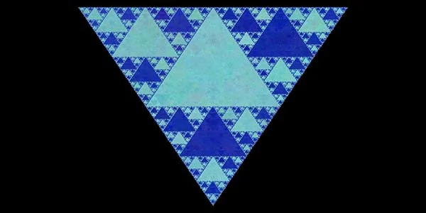
Learn how to create a colored version of the Siepinski-Triangle and many other fractals with recursive function calls.